Analysis of Boundary-Layer Transition Induced by Surface Imperfections

ABSTRACT

This work presents an experimental study on the effects of surface irregularities, specifically bumps and gaps, on boundarylayer transition. Transition mechanisms are investigated using hot-wire anemometry and a Preston tube. The experiments were conducted in the low acoustic noise and turbulence (LANT) wind tunnel at the Universidade de São Paulo, employing a flat-plate model with a variable insert capable of generating either a bump or a gap. The results show that bumps have a significantly stronger impact on the amplification of Tollmien-Schlichting waves than gaps, with amplification levels approximately four times higher for bumps at |h/δ∗| = 0.64. Furthermore, the critical height required to trigger bypass transition is lower for bumps than for gaps. In particular, bumps promote a rapid upstream shift of the transition location already at h/δ∗ = 1.29, whereas a comparable abrupt advancement toward the irregularity is observed for gaps only at h/δ∗ = −3.22. The data indicate that bypass transition induced by gaps is associated with Rossiter-type instabilities. In contrast, bypass transition over bumps appears to be governed by a distinct mechanism related to the growth of a downstream recirculation bubble, which induces an inflectional boundary-layer profile and gives rise to a high-frequency amplification band.

Keywords
Boundary-layer transition; Surface irregularities; Bumps; Gaps

INTRODUCTION

Viscous drag plays a significant role in diminishing aerodynamic efficiency, leading to several undesirable consequences, such as increased fuel consumption in aircraft, greater emissions of harmful gases, and elevated levels of aeroacoustic noise. Reneaux (2004) estimated that approximately 22% of an aircraft’s operating expenses were associated with fuel consumption when the average price of a barrel of oil was approximately 40 US dollars. Currently, this price has nearly doubled. One of the primary contributors to viscous drag is the turbulent boundary layer, which typically develops turbulence following the amplification of unstable modes that trigger the transition process. In two-dimensional boundary layers, the natural transition mechanism is governed by the growth of Tollmien-Schlichting (TS) waves, as demonstrated experimentally by Schubauer and Skramstad (1947). Moreover, TS waves can interact with surface irregularities, as highlighted by Crouch (2006), where these imperfections may include steps, bumps, and gaps. Crouch and Kosorygin (2020) further classified these irregularities based on their geometric characteristics. In reality, such surface imperfections can be observed on actual aircraft, including rivets, plate edges, dirt accumulation, and paint delamination. However, depending on the geometry and flow conditions, these irregularities can bypass the TS wave growth process, as noted by Beguet et al. (2017) and Crouch et al. (2022). In these cases, a different transition mechanism, distinct from TS waves, is responsible for triggering boundary-layer turbulence, as discussed by Saric et al. (2002).

The impact of surface irregularities on boundary-layer transition has been a subject of research since the last century. Tani et al. (1940) conducted experimental investigations on how a round transverse wire placed on a flat plate influences boundary-layer transition, analyzing how the wire diameter affects the transition Reynolds number. Similarly, Stuper (1949) examined forward-facing steps using a comparable methodology. A comprehensive review of this subject was provided by Dryden (1949). These studies indicated that an increase in roughness size leads to a reduction in the transition Reynolds number, meaning the transition onset shifts upstream, closer to the surface imperfection. Subsequently, Klebanoff and Tidstrom (1972) demonstrated that the recovery zone, which is the region immediately downstream of an imperfection (such as a transverse cylindrical rod), exhibits a distortion in the mean flow, leading to a destabilizing effect on the boundary layer. Cebeci and Egan (1989) developed a method that integrates an interactive procedure with the semi-empirical e^N approach, originally introduced by Ingen (1956) and Smith and Gamberoni (1956), to predict the transition location caused by a bump. The authors pointed out that the bump influences the critical frequency, which is the first-dimensional frequency to reach an integral growth beyond the transition threshold. Similarly, Nayfeh et al. (1988) conducted a related study and concluded that the bump modifies the transition-inducing frequency compared to the smooth surface case. Furthermore, they identified the bump height and its streamwise location as the key parameters affecting instability, along with the size of the separation bubble downstream of the obstacle, which also influences the transition point. According to Masad and Iyer (1994), this separation bubble significantly alters the transition location. They also reported that, for bump heights exceeding a certain threshold greater than the minimum height required for separation, the transition occurs abruptly over the bump itself. Regarding steps, Wang and Gaster (2005) developed an empirical tool based on experimental data to establish a relationship with the eN method. The correlation between the transition position and h/δ^∗ can be classified into three regions: (i) the presence of the step does not affect the transition; (ii) a transition range where the transition onset gradually shifts toward the step; and (iii) a saturation value of h/δ^∗, beyond which the transition occurs directly at the step.

The influence of gaps on transition follows a similar pattern to other surface imperfections. Some of the earliest experimental studies on this topic were conducted by Sarohia (1977) and Sinha et al. (1982). Sinha et al. (1982) investigated the effects of parameters such as gap depth and width, categorizing them as shallow or deep, open or closed. However, their findings did not provide conclusive information regarding the impact on the transition point. On the other hand, Sarohia (1977) established the conditions under which a cavity induces oscillatory motion. By employing the non-dimensional parameter (L/δ) √Reδ, they consolidated results from various flow conditions into a single curve. Although their research did not directly address the cavity’s influence on transition, the oscillation limits they identified bear a resemblance to the bypass transition thresholds later examined by Beguet et al. (2017) and Crouch et al. (2022). Regarding the role of gaps in boundary-layer transition, Beguet et al. (2017) developed an empirical relationship that links depth (D), length (L), and displacement thickness (δ^∗) to the N factor. Their results indicate that the evolution of the N factor can be divided into two regimes: a peak amplification over the gap (N_peak), which subsequently decays into a shifted-up curve parallel to the amplification observed in a smooth surface case (N_far). Additionally, they identified tripping limits, specifically for values of L/δ^∗ ≥ 18 and D/δ^∗ ≥ 2, where the transition occurs directly over the gap. Crouch et al. (2022) obtained a similar threshold and attributed this behavior to bypass transition. Furthermore, they detected high-frequency oscillations distinct from the TS wave range in a particular bypass transition case. Their experimental study modeled the impact of gap depth and length on transition and introduced an equation to estimate the shift in transition location in terms of ∆N as a function of gap length and aspect ratio. The aspect ratio determines a plateau where ∆N remains constant as L/δ∗ increases, a condition the authors refer to as the deep-gap limiting case.

From a computational perspective, Victorino et al. (2023) identified a connection between this bypass transition and unstable modes within the cavity, such as Rossiter and centrifugal modes. Their linear stability analysis revealed that the neutrality of the centrifugal mode is lower than that of the Rossiter mode, which aligns with the bypass transition limits reported by Beguet et al. (2017) and Crouch et al. (2022). In particular, the analysis of case C detected an unstable Rossiter mode with a frequency differing by only 4% from the experimental measurement by Crouch et al. (2022). Moreover, direct numerical simulations (DNS) demonstrated a non-linear interaction between the centrifugal and Rossiter modes, ultimately leading to transition.

This study examines the evolution of velocity disturbances and boundary-layer transition induced by various configurations of bumps and gaps in flow regimes governed by TS waves and bypass transition. The streamwise development of velocity fluctuation signals is investigated in both the time and spectral domains and is compared with predictions from linear stability theory (LST). Additionally, bumps and gaps of equivalent heights and depths are analyzed and contrasted. It is emphasized that the objective of the present experiments is not to establish the critical thresholds for bumps and gaps, which have been documented in the literature, but rather to ensure that the investigated configurations lie on each side of these thresholds and to compare the corresponding transition mechanisms. Understanding the distinct transition mechanisms involved in this phenomenon can provide deeper insights into the underlying physics, the relevant processes, and the associated flow regimes. Consequently, more accurate models for predicting the transition location can be formulated, enabling improved passive control of the laminar-turbulent transition. This, in turn, enhances aerodynamic efficiency and contributes to the development of more sustainable aircraft.

METHODOLOGY

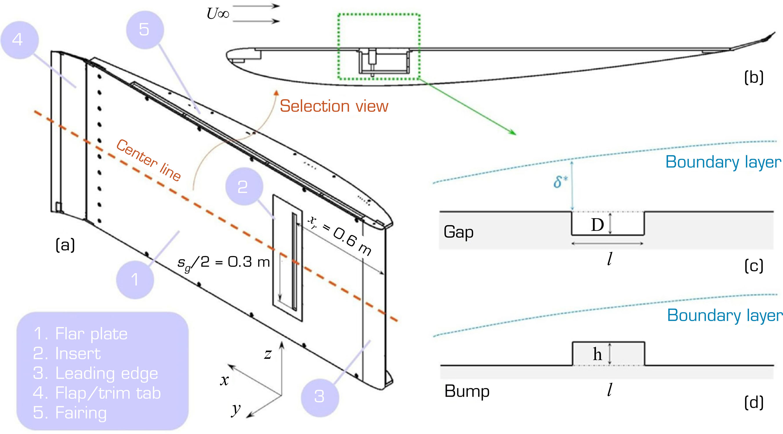
The test model consists of a flat aluminum plate with dimensions of 2,320 mm × 1,000 mm × 10 mm. It includes a tab and a flap to adjust the pressure gradient, which, for a Blasius profile, should ideally be as close to zero as possible. A schematic view of the model is presented in Fig. 1. The plate features an insert designed to accommodate a system that modifies the surface imperfection geometry, enabling the configuration of a smooth flat plate, a bump, or a gap. This system is positioned 600 mm from the model’s leading edge. The bump extends 30 mm in the flow direction and spans 600 mm, ensuring that the span is significantly larger than the other dimensions to minimize edge effects along the central line of the model. The bump height or gap depth has a displacement range of 20 mm, controlled by two stepper motors installed beneath this section. Additionally, the system allows for precise adjustments, with a maximum resolution of 20 µm for gap/bump movement.

Figure 1
Schematic characteristics of the model. (a) Isometric view; (b) Section view; (c and d) Details of a bump/gap within the boundary layer.

The instrumentation utilized in this study is detailed as follows. Velocity measurements, including both mean and fluctuating components, were performed using hot-wire anemometry (HWA). The anemometer employed is the AN-1002 from the A.A.Lab System, operating in constant temperature anemometry mode. The probe used as the sensing element is the Dantec Dynamics model 55P15, which is specifically designed for boundary-layer measurements. To position the probe accurately, a high-precision 3D Cartesian traverse was used, providing a movement resolution of 6.25 µm in the wall-normal direction (y). A wing covers the traverse rod to mitigate vortex shedding and prevent probe vibration that could contaminate the velocity fluctuation signal. This wing also houses additional sensors, including the Preston tube and a linear variable differential transformer distance sensor, which is used to determine the relative distance between the sensors and the plate. The anemometer output signal is transmitted to two data acquisition modules. The first module, a DAq-USB-6002 from National Instruments, is utilized for mean velocity measurements and features a 16-bit resolution with a sampling rate of up to 50,000 samples per second. The anemometer voltage readings are converted into velocity values through a calibration process using a static Pitot tube positioned inside the test section. The second module comprises a PXI-4496 board with 24-bit resolution, installed in a PXI-1042Q chassis, both from National Instruments. Due to its higher resolution, this module is responsible for acquiring the velocity fluctuation signal.

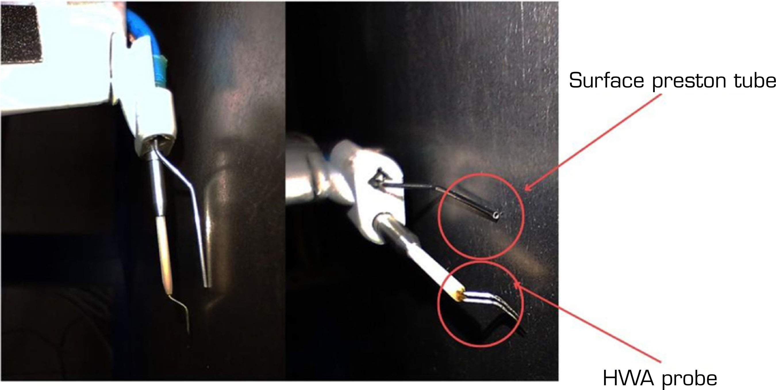
To estimate the transition location, a Preston tube is employed. This instrument measures the dynamic pressure of the flow over the wall. When a transition occurs, the velocity profile derivative changes, leading to an abrupt increase in the dynamic pressure measured by the instrument. Thus, the transition location is identified as the point where the Preston tube reading reaches its minimum value. The total pressure sensing element consists of a bent needle with a diameter of 0.9 mm, shaped similarly to the hot-wire probe. Additionally, the free-stream static pressure is measured using a Pitot-static tube mounted on the traverse wing. A Honeywell RSC differential pressure transducer is used for pressure data acquisition, ensuring a total error of less than 5 Pa. The tip of the three-dimensional positioner with both HWA probes and the Preston tube can be seen in detail in Fig. 2.

Figure 2
Detail of the HWA probe and the Preston tube in a typical measurement position.

The experiment comprised two distinct types of measurements: (i) a Preston tube sweep along the streamwise direction to determine the transition location; and (ii) hot-wire fluctuation velocity recordings at specific positions to analyze the disturbance evolution along the streamwise axis. Both types of measurements were conducted simultaneously. Furthermore, at each streamwise position x, the surface irregularity height was adjusted according to predefined values: h = 0, +0.8, +1.6, and +4 mm. From this point onward, h > 0 is defined as a bump and h < 0 as a gap. The free-stream velocity was maintained constant at U_∞ = 20 m·s^-1. The experimental grid was adapted based on the type of measurement being performed.

For the Preston tube measurements, two different streamwise spacings were employed: a finer spacing of 10 mm within the range 640 ≤ x ≤ 700 mm and a coarser spacing of 50 mm for the remainder of the model up to x = 1,900 mm. This setup allowed for the detection of potential backflow regions downstream of the bump, as previously reported by Klebanoff and Tidstrom (1972), Nayfeh et al. (1988), and Masad and Iyer (1994).

To characterize the disturbances, hot-wire measurements were conducted at x = 640 mm to capture the near-field effects of the irregularity, while the far-field disturbance evolution was recorded at positions ranging from 700 ≤ x ≤ 1,900 mm with a spacing of 100 mm. Regarding the wall-normal positioning, the hot-wire probe was placed at a fixed non-dimensional height $\eta =\mathrm{y}\sqrt{\frac{vx}{U}\mathrm{\infty }}\approx 1.23$, where the Blasius velocity profile corresponds to U/U_∞ = 0.4. This location was chosen as it coincides with the region of maximum TS wave amplitude.

Tunnel characterization

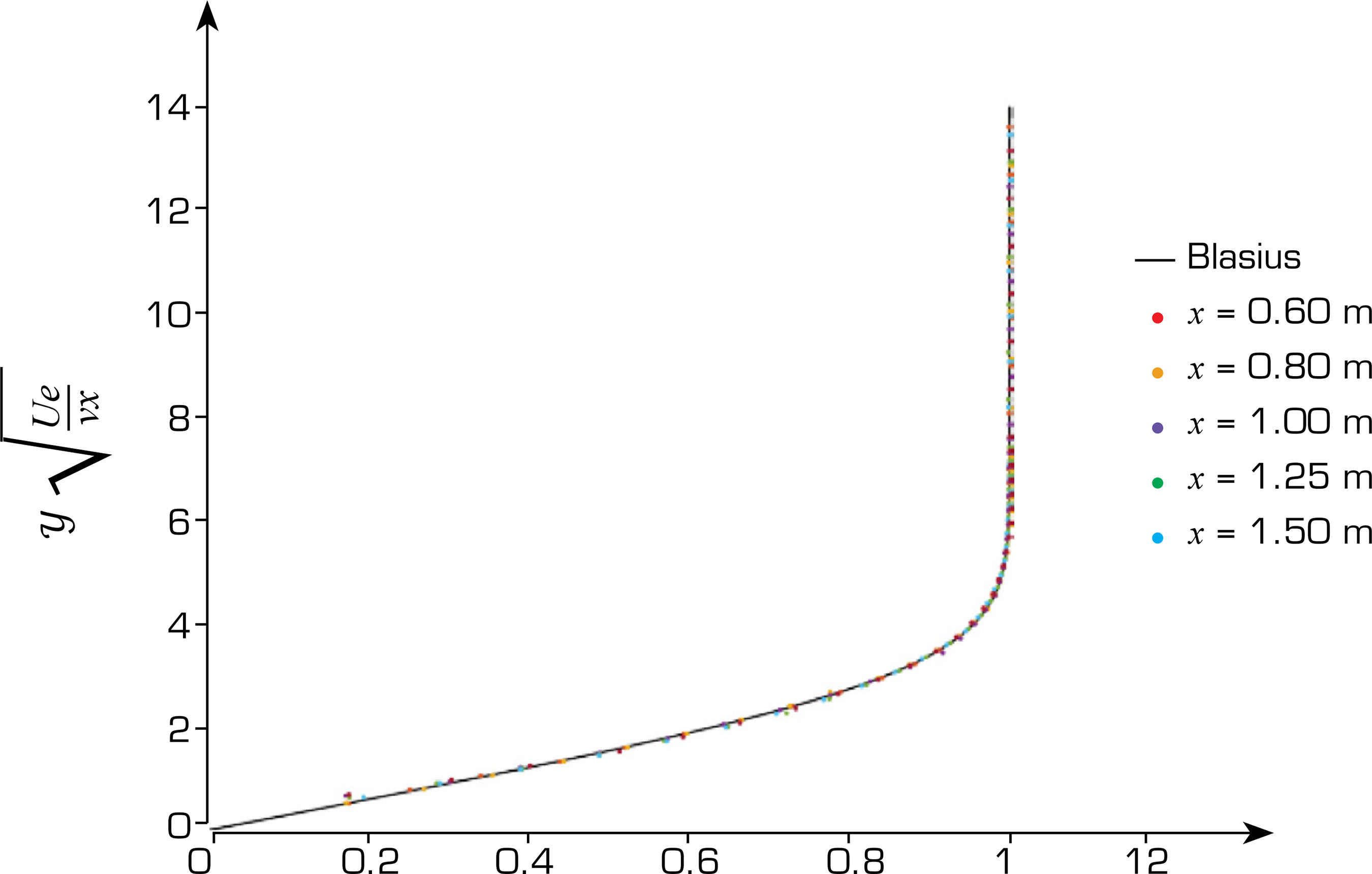
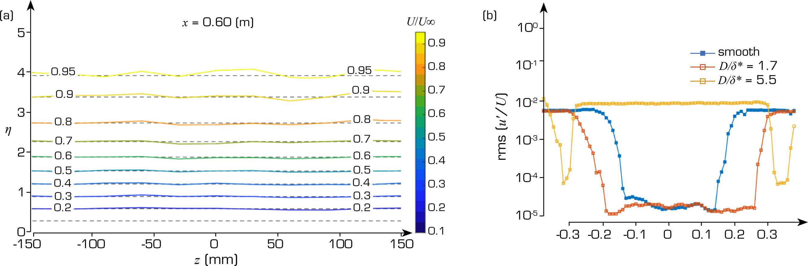
The experiments were conducted at a low acoustic noise and turbulence (LANT) wind tunnel, a closed-circuit wind tunnel located at Escola de Engenharia de São Carlos, Universidade de São Paulo. The test section has a square cross-section with dimensions of 1 m × 1 m and a length of 3 m. Further details about the wind tunnel can be found in Amaral et al. (2021). As indicated by its name, LANT is characterized by low acoustic noise and a low turbulence level in the free-stream, with a turbulence intensity of Tu = 0.03% (bandwidth 2-1,024 Hz) measured in an empty test section at a free-stream velocity of 20 m·s^-1. When the model was installed in the test section, the measured turbulence intensity was Tu = 0.054% (bandwidth 4-1,024 Hz) at a free-stream velocity of 27 m·s^-1. Additionally, the facility maintains a high level of flow uniformity, with velocity variations on the order of 1% of the free-stream velocity within a central area of 600 mm 600 mm in the test section. The mean velocity was calculated by averaging a 30-second time series acquired at each spatial location, using a sampling rate of 2,048 samples per second. To analyze the streamwise evolution, the profiles were measured at 600, 800, 1000, 1,250, and 1,500 mm. To recalculate the profiles with the correct distance to the wall, a procedure defined by Saric (1990) was used to compensate for the x position by computing a virtual leading edge distance value that matches the Blasius and the experimentally measured displacement thickness. Figure 3 depicts the mean normalized velocity profiles measured at different streamwise positions, compared to the theoretical Blasius profile. Figure 4a shows the contour of the normalized mean velocity profile at x = 0.60 m. One can see that the spanwise distribution of the boundary layer profiles, when compared to the theoretical profile, exhibits good agreement.

Figure 3
Comparison of mean velocity profiles with Blasius along the streamwise direction.

Regarding the disturbance velocity, the two-dimensionality of the boundary-layer disturbances was also investigated through the analysis of the fluctuation velocity signals. Measurements were taken at several spanwise positions in the range 0.38 m ≤ z ≤ 0.38 m, with a spacing of ∆z = 10 mm. This procedure was conducted for three different configurations: a smooth flat plate at x = 1.75 m, a flat plate with a shallow gap of depth D/δ^∗ = 1.7 at x = 1.20 m, and a deeper gap with D/δ^∗ = 5.5 at x = 0.65 m. The Reynolds number for these tests was U∞/ν = 1.75 × 10⁶·m⁻¹. Figure 4b presents the root mean square (RMS) of the disturbance velocity, normalized by the free-stream velocity, for the three configurations.

Figure 4
Two-dimensionality of the boundary layer. (a) Mean velocity profiles at x = 0.60 m (Blasius in dashed); (b) RMS of the disturbance velocity in three conditions: smooth (blue) and past gaps, affecting the TS (orange), and causing bypass transition (yellow).

Figure 5 compares experimental results with DNS presented by Himeno et al. (2023). The simulation was performed using the following parameters: Reδ^∗ = 1500 at x = xg and Mach number M = 0.1, closely matching the experimental conditions where Reδ^∗ ≈ 1,600 at x = xg and M = 0.08. The TS waves in the DNS were triggered by introducing a localized wave packet. Figure 5a presents a comparison of the spatial growth of selected modes, while Fig. 5b displays the comparison of the numerical results with the frequency spectrum obtained experimentally. The DNS exhibited good agreement with the experimentally acquired data.

Figure 5
Growth of TS waves compared to DNS computed by Himeno et al. (2023). (a) Selected frequencies, dominant frequency between DNS and experiments; (b) Streamwise evolution of the spectra.

RESULTS

Table 1 summarizes the information regarding surface irregularities, the transition location, and the transition mechanism, which will be further analyzed. The transition was determined by the Preston tube, as shown in Fig. 6. When the transition occurs, the dynamic pressure at the wall rises from the smooth-case level to a higher pressure level. An example of this behavior is shown in the curve corresponding to bump B1 (h/δ^∗ = 0.64), in which the dynamic pressure soars from x = 1.6 m. This is caused by the laminar-turbulent transition. Nevertheless, the curves near the roughness element (0.64 ≤ x ≤ 0.8 m) show some nuances. Those nuances are not related to a change in the mean profiles due to the laminar-turbulent transition, but rather to a change in the velocity profile due to the interference of the surface irregularity in the mean flow. There is a systematic trend in which gaps increase the dynamic pressure at the wall, whereas the opposite occurs with the bumps. In this manner, the gaps tend to distort the mean flow in a way similar to a favorable-pressure-gradient profile, fuller close to the wall, while bumps alter the profiles to an adverse-pressure-gradient-like one. Far downstream, the dynamic pressure eventually falls to the smooth-case reference when no laminar-turbulent transition occurs. Dynamic pressures lower than the smooth flat-plate curve, observed in bump cases, will be further discussed later.

Figure 6
Preston tube data for all cases.

For the free-stream velocity considered, the transition was not reached in the smooth case, as well as in one of the cases with a gap, due to the insufficient length of the flat plate to attain the transition Reynolds number. An additional experiment conducted at a higher velocity indicated that the transition Reynolds number for the smooth flat plate occurs at Rex = 2.4 × 10⁶. Nonetheless, laminar-turbulent transition was observed in cases G2, G3, B1, B2, and B3. These results suggest that, for a constant Reδ^∗, a bump is more destabilizing than a gap of the same height relative to the displacement thickness. A comparison between the transition Rex and the semi-empirical model proposed by Wang and Gaster (2005) for backward-facing steps demonstrated reasonable agreement. The transition Reynolds numbers for cases B1 and B2 were found to be Rex = 1.86 × 10⁶ and 0.82 × 10⁶, respectively, whereas the values extracted from the curve in Wang and Gaster (2005) for equivalent backward-facing step heights were Rex = 1.86 × 10⁶ and 1.01 × 10⁶.

Effect of bumps and gaps on TS waves

Next, the streamwise evolution of the fluctuation velocity is presented. The signals were analyzed in both time and frequency-domains. Welch’s method was employed to compute the power spectral density (PSD) for the frequency domain analysis (Bendat and Piersol 2010). This method estimates the PSD by averaging the PSDs of the entire signal divided into blocks. In total, the PSD of the original time series is the result of the ensemble of 179 segments with 50% overlap. This approach smooths the spectrum at the cost of reducing the bandwidth (Δf = 2 Hz). A Hanning window function was also applied to each segment to mitigate side-lobe leakage. Once the ensemble-averaged PSD was obtained, the amplitude of each frequency component was determined by taking its square root. The sampling rate fs was 8,192 samples per second, enough to capture eventual high-frequency Rossiter modes. The anti-aliasing filter is embedded in the Peripheral Component Interconnect eXtensions for Instrumentation (PXI) boards and automatically sets the cut-off frequency as fc = 0.49fs (fc ≈ 4,014 Hz).

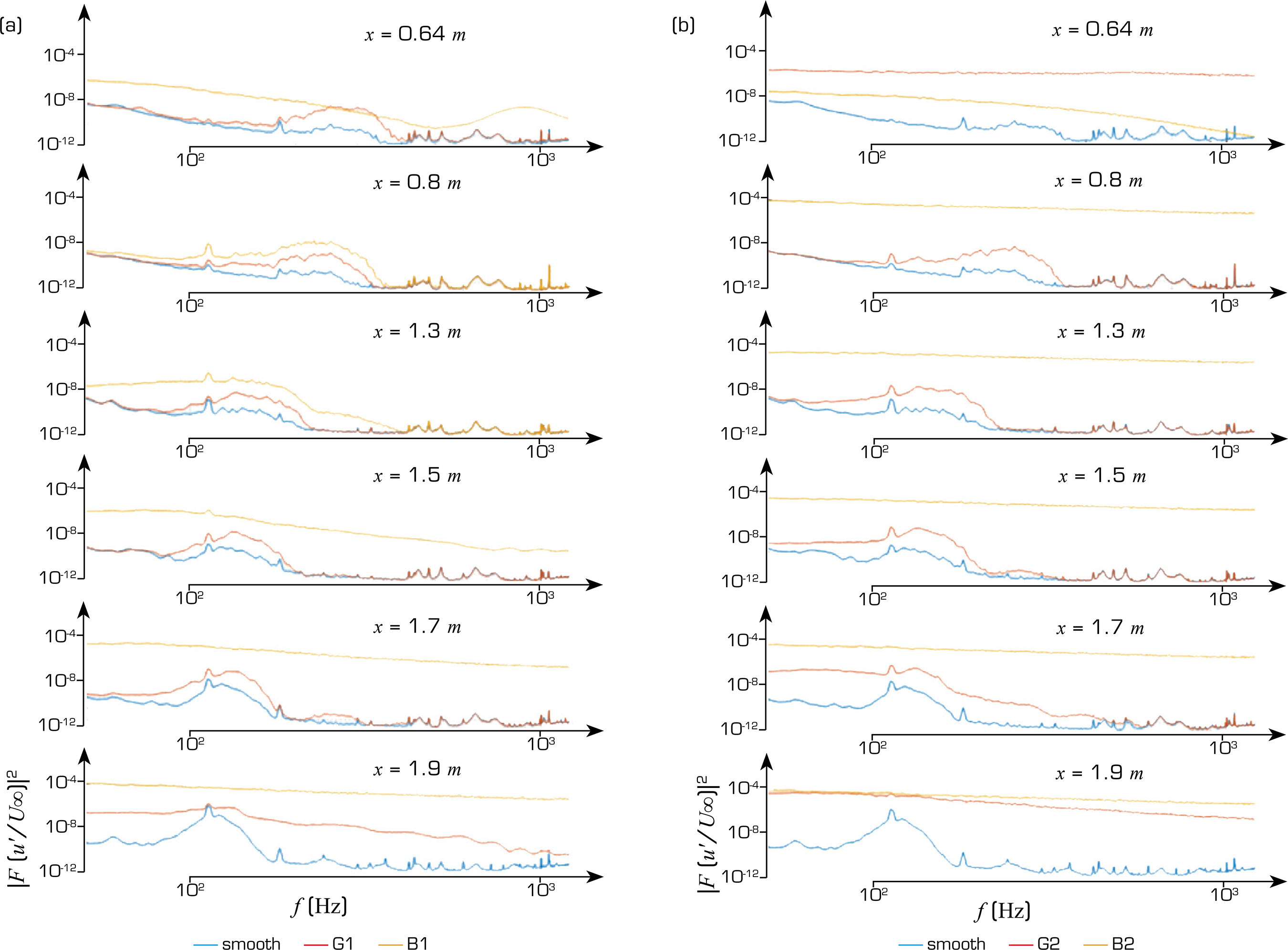
Figure 7 shows the streamwise evolution of the power spectra for the case pairs G1-B1 and G2-B2, with comparisons to the smooth reference case (S). Similarly, Fig. 8 presents amplitude contour maps as functions of the Reynolds number Reδ^∗ and the non-dimensional frequency F = 2π fν/U²_∞ × 10⁶, juxtaposed with the theoretical neutral limits (dashed) obtained from the solution of the Orr-Sommerfeld equation (OSE) according to Juniper et al. (2014). The unstable region occurs within the neutral limits. In each of the spectral figures, the smooth case (S) is displayed in the middle row to facilitate comparison, while each column corresponds to the gap and bump cases, respectively. The spectral content can be broadly divided into two frequency regions: a low-frequency range (f ≤ 50 Hz), which exhibits high amplitude, and the higher-frequency range. Although the low-frequency band contains a significant portion of the total oscillatory energy, its amplitude remains nearly constant along the streamwise direction, except in regions where transition to turbulence occurs. This low-frequency content is commonly attributed to the background noise of the boundary layer, as noted by Wang and Gaster (2005). Additionally, the spectra display a few distinct peaks caused by electrical noise. However, these noises do not interfere with the interpretation of the results.

Figure 7
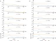
Amplitude spectra of HWA signals collected in a streamwise sweep for different irregularity configurations. (a) Cases B1, G1, and S; (b) Cases B2, G2, and S.

Figure 8
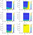
Amplitude contours (log scale) compared with the LST for some irregularity configuration: (a) G1; (b) B1; (c) and (d) S; (e) G2; (f) B2.

Firstly, examining the smooth case (S), a bell-shaped frequency band can be observed amplifying along the streamwise direction. This band corresponds to the range of unstable TS wave frequencies, as also depicted in Fig. 8. As predicted by LST, the dimensional frequency range varies with Reδ^∗ (i.e., with x), shifting from higher frequencies (200 ≤ f [Hz] ≤ 400) in the upstream region to lower frequencies (70 ≤ f [Hz] ≤ 200) further downstream.

Next, for the pair of cases with | h/δ^∗|= 0.64 (G1 and B1), the spectral evolution differs significantly between the two configurations. At the most upstream measurement station (x = 0.64 m), the gap (G1) affects primarily the TS band, slightly amplifying its components. In contrast, the bump (B1) exhibits substantially higher amplitudes in a broader frequency range (10-600 Hz). Moreover, a high-frequency bulge appears approximately at 909 Hz, indicating an additional amplification mechanism. Later, a more in-depth study regarding this particular topic will provided.

According to Fig. 8, cases G2 and B2 display even more pronounced differences. For G2, the spectral content in the gap’s near-field is nearly flat, with significantly elevated amplitudes. However, these high-amplitude oscillations rapidly decay downstream. This behavior suggests that the flow over the gap undergoes oscillatory motion that is not sustained within the boundary layer further downstream, most likely because the excited frequencies lie outside the unstable TS range. As a result, the TS wave amplitudes in G2 are greater than those observed in the smooth case (S), which explains why the transition occurred at x = 1.8 m in case G2, whereas it did not occur in the smooth case within the length of the model. This behavior can be explained by the hypothesis that, in this particular case, turbulence is generated inside the gap’s mixing layer and is convected into the boundary layer. Frequencies outside the unstable TS band stabilize; however, the ones that match the unstable range amplify the TS, shifting the transition location to x = 1.8 m as a consequence.

On the other hand, case B2 revealed a strong destabilization of the boundary layer induced by the bump, leading to an abrupt transition. Due to the limited number of measurements in this region, it remains unclear whether the transition mechanism was driven by the amplification of TS waves or bypassed by an alternative route.

Figure 9 presents the amplification factor ln(A/AS) relative to the smooth reference case for configurations G1 (Fig. 9a) and B1 (Fig. 9b). For case G1, the amplified frequency band is clearly associated with TS waves, with amplification factors on the order of ln(A/AS) ≈ 2. Similarly, case B1 exhibited an amplification factor within the LST unstable band, with a significantly greater value, ln(A/AS) ≈ 3.5. In contrast, there is a different behavior in the rectangular bump near-field. Immediately downstream of the roughness element, the amplified frequencies are centered at a higher frequency (F ≈ 250) and present a broader band compared to the smooth counterpart. This non-dimensional frequency corresponds to the bulge, approximately 909 Hz, depicted in Fig. 7b. This broadband amplification outside the expected unstable range from LST may indicate the presence of a locally modified boundary layer induced by the bump.

Figure 9
(a and b) Contours of amplification factor relative to the Smooth case, ln (A/AS), compared with the LST neutral limits (dashed); (c) Inflectional profile with m = 0.09 used for calculating the branch II (blue) depicted in (b).

The observed spectral behavior in case B1 is consistent with the development of an inflectional boundary-layer velocity profile downstream of the bump, as exhibited in Fig. 9b. This assumption is adopted because the rectangular bump geometry imposes a local adverse pressure gradient, which in turn causes a flow separation. This topological flow feature is reported in the literature as the so-called recovery region (Himeno et al. 2024; Klebanoff and Tidstrom 1972).

The Preston tube dynamic pressure at x = 0.64 m for case B1 is lower than that of the smooth case, corroborating this assumption. Additionally, the recirculation length downstream of the bump was estimated through extrapolation of the numerical results from Himeno et al. (2024) with a value Lrecirc ≈ 16.6 δ^* ≈ 18 mm, suggesting that, in case B1, the hot-wire probe was positioned inside the separation caused by the irregularity, as the flow reattaches at x = 0.648 m. This led to perform an analysis involving LST and an inflectional boundary-layer profile, as below.

It is known that the pressure gradient alters the Orr-Sommerfeld stability characteristics (Schlichting and Gersten 2000), widening the unstable frequency band mostly due to a shift of the second branch (upper boundary) of the neutral stability curve toward higher frequencies. To support this interpretation, a linear stability analysis was performed using a Falkner-Skan profile with pressure-gradient parameter m = 0.09, representative of the inflectional flow induced by the rectangular bump, similar to what was experimentally measured by Klebanoff and Tidstrom (1972). The value of m is close to the lower limit for which Falkner-Skan solutions exist and thus represents a limiting case of adverse pressure-gradient flow. For convenience, only the second branch of the neutral stability curve was computed and is shown in Fig. 9b. It must be stressed that inflectional profiles (m < 0) exhibit an increased local displacement thickness δ^*, and consequently a higher local Reynolds number Reδ^∗. This higher local Reynolds number was employed for the LST calculations; however, to enable a direct comparison with the smooth-wall reference case, the second branch of the stability diagram is projected onto the Reynolds-number axis based on the smooth-wall displacement thickness in Fig. 9b, effectively providing a reference-consistent representation of the instability characteristics. The branch II computed lies quite near the amplified bulge, approximately 909 Hz (Fig. 7a), which in non-dimensional terms corresponds to F ≈ 250 (Fig. 9b). This is consistent, as branch II typically corresponds to the region of maximum TS-wave amplitude. Further downstream of the roughness element, the boundary-layer profile gradually recovers toward a Blasius-type profile, and the stability characteristics revert toward those of the canonical flat-plate diagram. In this region, the amplification factors within the TS-frequency band increase to approximately ln(A/AS) ≈ 3.5, while after transition, they attain values close to ln(A/AS) ≈ 8, reflecting the onset of nonlinear growth and breakdown.

Bypass transition regime

Bypass transition in gaps

Figure 10 illustrates the streamwise evolution of the fluctuation velocity spectrum for case G3, obtained using the same methodology as previously described. The spectra exhibit characteristics typical of turbulent flow, with high-amplitude spread throughout a wide range of frequencies. For the sake of comparison, the RMS normalized by the free-stream velocity of the velocity signals u′_RMS/U_∞ were 0.008 and 0.16 for S and G3, respectively, about 20 times greater. A sharp spectral peak is observed, with relatively high amplitude and frequency compared to the TS band of the smooth flat plate case at similar streamwise locations. This peak is attributed to a Rossiter mode. The corresponding non-dimensional frequency, fL/U = 0.78, is close to the second Rossiter mode (R₂), as predicted by the semi-empirical formula of Rossiter (1966).

Figure 10
Evolution of the velocity disturbance spectrum along the flow direction for the G3 case (h/δ∗ = −3.22) showing the presence of the Rossiter mode near the gap.

Downstream of the gap, the amplitude of the Rossiter mode decays. This occurs for the following reason. The Rossiter mode oscillations develop over the mixing layer inside the cavity opening. Far downstream, part of this motion spills outside the cavity; however, the shear layer reattaches, forming a boundary layer. The frequency of the residual oscillation is considerably higher than the unstable band predicted by the local theory. Hence, those oscillations diminish downstream in a quite sharp manner. Nonetheless, this high-amplitude motion promotes sufficient energy for self-sustained turbulence, causing the boundary layer to undergo laminar-turbulent transition. Victorino et al. (2023) reported that centrifugal instabilities rise before the Rossiter mode and are necessary to compose the laminar-turbulent process; however, the present experiment does not allow the investigation of this type of instability, which is essentially, is three-dimensional and is contained mostly inside the cavity. In any case, the experiment indicates that the Rossiter instability is a fundamental mechanism, causing a cavity-induced transition process.

Figure 6, which presents Preston tube data, also corroborates that the case G3 exhibits a turbulent boundary layer immediately downstream of the gap. This is reflected in the Preston tube curve, which depicts a behavior similar to the smooth case curve, albeit at a higher dynamic pressure level, indicating a fully developed turbulent state at the cavity trailing edge.

Bypass transition in bumps

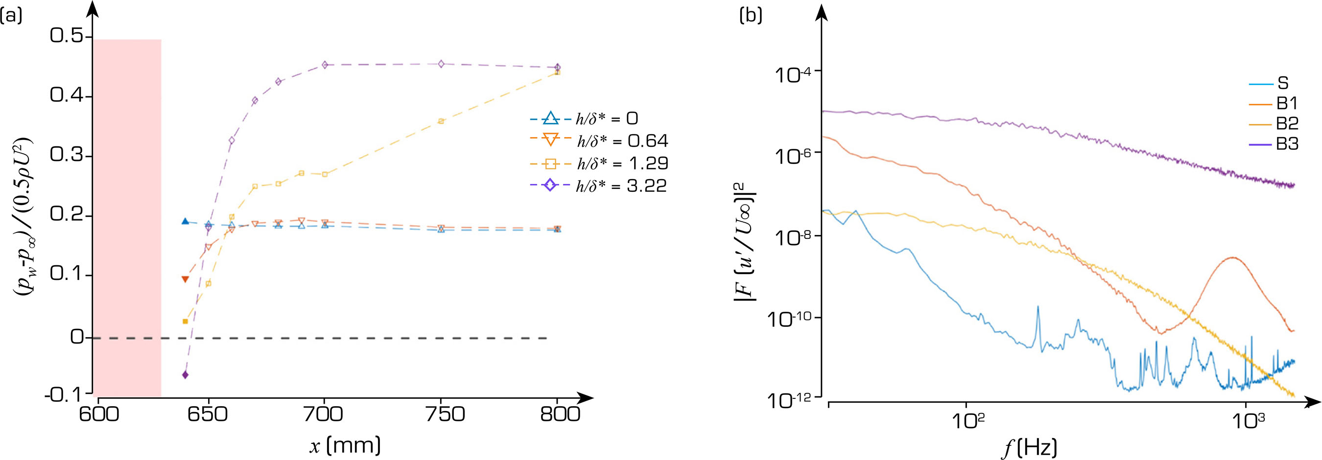
In contrast to gaps, where the Rossiter mode governs the bypass transition, the bypass transition observed for bumps is intrinsically linked to the development and growth of a downstream recirculation bubble. Preston tube measurements provide evidence of this mechanism. Immediately downstream of the bump, the wall dynamic pressure exhibits a pronounced reduction, reaching negative values in case B3. This behavior is a strong indication of flow separation at the bump’s trailing edge. This observation is consistent with the findings of Himeno et al. (2024), Nayfeh et al. (1988), and Masad and Iyer (1994), who reported that separation bubbles of this nature have a substantial impact on the transition process. As shown in Fig. 11a, the extent and intensity of this low-pressure region increase systematically with bump height, suggesting a progressive growth of the recirculation bubble as h/δ^∗ increases. This observation supports the hypothesis that the bump-induced bypass transition is controlled not merely by the presence of separation, but by the growth and strengthening of the recirculation bubble, which substantially modifies the local boundary-layer structure. Spectral evidence further reinforces this interpretation. The full-colored markers in Fig. 11a represent the positions where Fig. 11b provides a zoomed-in view of the PSD from all bump cases. The PSD of case B1 was previously discussed. Concerning case B2, the PSD shows a turbulent-like spectrum, however, with low amplitudes and RMS. It is believed that this occurred because the position where the signal was measured (y/δ^∗ ≈ 0.6) was close to the recirculation core that occurs roughly at the mid-height of the rectangular bump (h/δ^∗)/2 = 0.645. Near the recirculation center, the velocity is reduced and presents two components, which are not proper for a single-sensor hot wire. Finally, as B3 shows a spectrum that resembles a turbulent one. In this particular case, the dynamic pressure at the wall progressively goes from negative values to the turbulent level in the streamwise direction.

Figure 11
Data comparison of the smooth and bump cases (S, B1, B2, and B3). (a) Streamwise distribution of dynamic pressure at the wall collected by the Preston tube; (b) Frequency spectra of the respective cases at x = 0.64 m (filled markers).

A detailed examination of the velocity fluctuation signals reveals that this high-frequency band is associated with intermittent, non-periodic events rather than sustained oscillations. As illustrated in Fig. 12, these events consist of a large-amplitude velocity excursion followed by the emission of a high-frequency wave packet. The corresponding spectrogram and wavelet analyses confirm that these packets are localized in time and centered at approximately the same frequency observed in the spectra, pointing to an instability mechanism related to unsteady vortex shedding or shear-layer dynamics at the trailing edge of the recirculation bubble. As the bump height increases further (case B3), the recirculation bubble grows sufficiently to promote immediate breakdown to turbulence. In this case, the boundary layer downstream of the bump exhibits spectral characteristics typical of fully turbulent flow, with broadband high-amplitude fluctuations and no identifiable TS-dominated growth stage. This behavior contrasts with the gap-induced bypass transition, where high-frequency oscillations decay rapidly downstream and act primarily as a trigger for turbulence rather than as a sustained destabilizing mechanism. Taken together, these results indicate that the bypass transition over bumps is fundamentally controlled by the growth of the recirculation bubble downstream of the roughness element. As the bubble enlarges, it induces increasingly inflectional velocity profiles, which substantially enhance the TS-wave amplification process. This mechanism explains why bumps require significantly smaller critical heights than gaps to promote abrupt transition.

Figure 12
(a) Detail of the velocity fluctuation time series of case B1 showing the excursion-packet emission structure. (b) Spectrogram of the case B1 time series. (c) Wavelet of the case B1 showing the distribution of the amplitude of the structure through time.

CONCLUSION

This paper presented an experimental investigation into the stability and transition of a boundary layer subjected to an interchangeable surface irregularity capable of forming either a bump or a gap. To characterize the transition process and quantify the influence of surface irregularities on TS wave development, measurements were obtained using HWA and a Preston tube. First, strong agreement between the experimental results and LST was observed, confirming that the TS unstable frequency range matched the theoretical predictions. Second, a comparative analysis between bumps and gaps with equivalent height relative to the local displacement thickness and Reynolds number revealed that bumps exert a more destabilizing influence. This effect was evident through the enhanced amplification of TS waves and a larger upstream shift of the transition location, as quantified by the calculation of the amplification factors. Third, bypass transition mechanisms were identified for both types of irregularities. For the gap, a Rossiter mode instability was detected, with a non-dimensional frequency close to the second mode (R₂) as predicted by the semi-empirical models of Block (1976) and Rossiter (1966). This observation is consistent with the numerical findings of Victorino et al. (2023), which also identified the Rossiter mode as a transition mechanism. For the bump, the critical height required to induce bypass transition was found to be smaller than the corresponding critical depth for a gap. Preston tube measurements and spectral analysis suggested the presence of a separation bubble near the bump’s trailing edge, indicating its role in promoting bypass transition. This phenomenon aligns with previous findings by Nayfeh et al. (1988) and Masad and Iyer (1994), who reported a strong influence of separation bubbles on the transition process. The dataset is not sufficient for a full empirical correlation between the effects of bumps and gaps. Therefore, further work with a more complete spacing in the parametric space will aim to establish a correlation. In conclusion, for surface roughness elements of similar dimensions, bumps are more detrimental to boundary-layer stability than gaps. Therefore, in applications requiring high aerodynamic efficiency and minimal drag, such as in the design of streamlined surfaces, it is preferable to favor configurations with gaps over those with bumps.

ACKNOWLEDGEMENTS

Not applicable.

• FUNDING
  Fundação de Amparo à Pesquisa do Estado de São Paulo
  Grant No: 2024/21737-6
  Coordenação de Aperfeiçoamento de Pessoal de Nível Superior
  Grant No: Finance Code 001
  Conselho Nacional de Desenvolvimento Científico e Tecnológico
  Grant No: 307956/2019-9
  Financiadora de Estudos e Projetos
  Grant No: 01.09.0334.04
  Fundação de Amparo à Pesquisa do Estado de São Paulo
  Grant No: 2019/15366-7
  The Boeing Company
  Grant No: 2021-GT-353
  US Air Force Office of Scientific Research
  Grant No: FA9550-18-1-0112 and FA9550-23-1-0030
• DECLARATION OF USE OF ARTIFICIAL INTELLIGENCE TOOLS
  The authors declare that no artificial intelligence tools were used in the preparation, writing, data analysis, or review of this manuscript.
• Peer Review History:
  Single Blind Peer Review.

DATA AVAILABILITY STATEMENT

All data sets were generated or analyzed in the current study.

References

• Amaral FR, Serrano Rico JC, Bresci CS, Beraldo MM, Victorino VB, Gennaro EM (2021) The low acoustic noise and turbulence wind tunnel of the University of São Paulo. Aeronaut J 1-45. https://doi.org/10.1017/aer.2021.80
  » https://doi.org/10.1017/aer.2021.80
• Beguet S, Perraud J, Forte M, Brazier JP (2017) Modeling of transverse gaps effects on boundary-layer transition. J Aircr 54:794-801. https://doi.org/10.2514/1.C033647
  » https://doi.org/10.2514/1.C033647
• Bendat JS, Piersol AG (2010) Random data, analysis and measurement procedures. New York: John Wiley and Sons. https://doi.org/10.1002/9781118032428
  » https://doi.org/10.1002/9781118032428
• Block PJW (1976) Noise response of cavities of varying dimensions at subsonic speeds. NASA Tech Note NASA-TN-D-8351:1-32.
• Cebeci T, Egan DA (1989) Prediction of transition due to isolated roughness. AIAA J 27(7):870-875. https://doi.org/10.2514/3.10194
  » https://doi.org/10.2514/3.10194
• Crouch JD (2006) Instabilities in boundary-layer flows and their role in engineering. Paper presented 2006 IUTAM Symposium on One Hundred Years of Boundary-layer Research. IUTAM; DLR-Göttingen, Germany. https://doi.org/10.1007/978-1-4020-4150-1_10
  » https://doi.org/10.1007/978-1-4020-4150-1_10
• Crouch JD, Kosorygin VS (2020) Surface step effects on boundary-layer transition dominated by Tollmien-Schlichting instability. AIAA J 58(7):2943-2950. https://doi.org/10.2514/1.J058518
  » https://doi.org/10.2514/1.J058518
• Crouch JD, Kosorygin VS, Sutanto MI, Miller GD (2022) Characterizing surface-gap effects on boundary-layer transition dominated by Tollmien-Schlichting instability. Flow 1-14. https://doi.org/10.1017/flo.2022.1
  » https://doi.org/10.1017/flo.2022.1
• Dryden HL (1949) Review of published data on the effect of roughness on transition from laminar to turbulent flow. Natl Advis Comm Aeronaut 477-482. https://doi.org/10.2514/8.2693
  » https://doi.org/10.2514/8.2693
• Himeno FH, Carvalho A, Medeiros M (2024) Analyses of Reynolds and Mach number effects on Tollmien-Schlichting wave-bump interaction in subsonic flows. J Fluid Mech 998 A11. https://doi.org/10.1017/jfm.2024.675
  » https://doi.org/10.1017/jfm.2024.675
• Himeno FH, Carvalho AEB de, Medeiros MA. Effect of small rectangular bumps on the amplification of Tollmien-Schlichting waves. Paper presented 2023 AIAA Aviation Forum. AIAA; San Diego, USA. https://doi.org/10.2514/6.2023-3996
  » https://doi.org/10.2514/6.2023-3996
• Ingen J van (1956) A suggested semi-empirical method for the calculation of the boundary-layer transition region. University of Technology, Department of Aerospace Engineering. Rep UTH-74.
• Juniper MP, Hanifi A, Theofilis V (2014) Modal stability theory: lecture notes from the flow-nordita summer school on advanced instability methods for complex flows, Stockholm, Sweden, 2013. Appl Mech Rev 66(2):024804. https://doi.org/10.1115/1.4026604
  » https://doi.org/10.1115/1.4026604
• Klebanoff PS, Tidstrom KD (1972) Mechanism by which a two-dimensional roughness element induces boundary-layer transition. Phys Fluids 15:1173-1178. https://doi.org/10.1063/1.1694065
  » https://doi.org/10.1063/1.1694065
• Masad JA, Iyer V (1994) Transition prediction and control in subsonic flow over a hump. Phys Fluids 6(1):313-327. https://doi.org/10.1063/1.868086
  » https://doi.org/10.1063/1.868086
• Nayfeh AH, Ragab SA, Al-Maaitah AA (1988) Effect of bulges on the stability of boundary-layers. Phys Fluids 31(4):796-806. https://doi.org/10.1063/1.866815
  » https://doi.org/10.1063/1.866815
• Reneaux J (2004) Overview on drag reduction technologies for civil transport aircraft. Paper presented 2004 European Congress on Computational Methods in Applied Sciences and Engineering. ECCOMAS; Jyväskylä, Finland.
• Rossiter JE (1964) Wind-tunnel experiments on the flow over rectangular cavities at subsonic and transonic speeds. Aeronautical Research Council Rep Mem 3438. London: Ministry of Aviation.
• Saric WS (1990) Low-speed experiments: requirements for stability measurements. In: Hussaini MY, Voigt RG, editors. Instability and transition. ICASE/NASA LaRC series. New York: Springer. p. 162-174. https://doi.org/10.1007/978-1-4612-3430-2_20
  » https://doi.org/10.1007/978-1-4612-3430-2_20
• Saric WS, Reed HL, Kerschen EJ (2002) Boundary-layer receptivity to freestream disturbances. Annu Rev Fluid Mech 34(1):291-319. https://doi.org/10.1146/annurev.fluid.34.082701.161921
  » https://doi.org/10.1146/annurev.fluid.34.082701.161921
• Sarohia V (1977) Experimental investigation of oscillations in flows over shallow cavities. AIAA J 15:984-991. https://doi.org/10.2514/3.60739
  » https://doi.org/10.2514/3.60739
• Schlichting H, Gersten K (2000) Boundary-layer theory. 8th ed. New York: Springer. https://doi.org/10.1007/978-3-642-85829-1
  » https://doi.org/10.1007/978-3-642-85829-1
• Schubauer GB, Skramstad HK (1947) Laminar boundary-layer oscillations and stability of laminar flow. J Aeronaut Sci 14: 69-78. https://doi.org/10.2514/8.1267
  » https://doi.org/10.2514/8.1267
• Sinha SN, Gupta AK, Oberai MM (1982) Laminar separating flow over backsteps and cavities part II: cavities. AIAA J 20: 370-375. https://doi.org/10.2514/3.7918
  » https://doi.org/10.2514/3.7918
• Smith AMO (1956) Transition, pressure gradient and stability theory. Douglas Aircraft Co. Report ES 26388.
• Stüper J (1949) The influence of surface irregularities on transition with various pressure gradients. Canberra: Department of Supply and Development, Division of Aeronautics.
• Tani I, Hama R, Mituisi S (1940) On the permissible roughness in the laminar boundary-layer. J Aeronaut Res Inst Tokyo 199.
• Victorino VB, Aguirre FO, Medeiros MAF (2023) Gap induced boundary-layer transition. AIAA Aviation Forum 1-14. https://doi.org/10.2514/6.2023-3997
  » https://doi.org/10.2514/6.2023-3997
• Wang YX, Gaster M (2005) Effect of surface steps on boundary-layer transition. Exp Fluids 39:679-686. https://doi.org/10.1007/s00348-005-1011-7
  » https://doi.org/10.1007/s00348-005-1011-7

Edited by

• Section editor:
  SungKi Jung https://orcid.org/0000-0002-0665-8191

Publication Dates

• Publication in this collection
  20 July 2026
• Date of issue
  2026

History

• Received
  15 Nov 2025
• Accepted
  17 Apr 2026