Methodology for the Thermal Models Development of the Brazilian Inertial System

ABSTRACT

This work presents a methodology to produce the thermal models of the Inertial Navigation System (Sistema de Navegação Inercial), being developed along with its host micro-satellite launch vehicle by the Brazilian Air Force (Força Aérea Brasileira). The rationale is built upon (i) knowledge gathering about the modelling and identification subject and the intended use of the thermal models, (ii) selection of the model’s “box color,” (iii) determination of the theoretical and/or the experimental setup, and (iv) definition of the necessary procedures, which comprise steps, rules, and metrics for selecting and validating the models. Given the “intended use” aimed at facilitating component replacement and parameter tuning, the light-gray box approach is selected, where each component is modelled individually and subsequently grouped hierarchically as submodels. The theoretical setup utilizes the MATLAB + SIMSCAPE environment, while the experimental setup relies on the open-source electronics platform named Arduino. Finally, the procedure is defined whereby the models’ parameters are progressively tuned, based on comparisons between simulation data and experimental measurements, following the progressive aggregation of the system components. The results demonstrate a good correlation between both data and measurements across all aggregation phases. Future work includes complex scenarios and rocket launch campaign results.

Keywords
Thermal analysis; Inertial navigation; Hierarchical modelling; System Identification; SISNAV; MATLAB

INTRODUCTION

System modelling and identification (M&I)

The etymology of the word “engineering” (and its correlates “engine” and “engineer”) and its historical development are particularly interesting, as they convey meanings generally associated with the design and creation of devices or machines (McFadden 2017). From the perspective of modern control theory, it is evident that this design process is implicitly grounded in system modelling (SM) and system identification (SI) techniques.

The term “system identification” was coined by Lofti Zadeh in 1962, as noted in the Ljung (1996) article “Development of System Identification”, being mostly popularized in the control community. System identification complements SM, with both fields owning specific techniques and procedures, thus offering a pathway to practical applications in the real world.

Models can range from intuitive abstractions and graphical representations to mathematical frameworks that may or may not embed software and lookup tables (Ljung 1999). A key decision during the SM procedure involves selecting a compatible “colored box” (white, light-gray, dark-gray, or black one, as categorized by Isermann and Münchhof (2010) or “boxes” (in a hierarchical approach) for the M&I subject. To determine that, it is essential to understand not only the actual system but also the model’s intended application: Is a straightforward linear mathematical white box sufficient? Is a physical description incorporating nonlinearities necessary, due to complex or critical use cases?

Researchers may possess varying degrees of physical or experimental knowledge regarding the constitution of the full or decomposed system to be modelled or identified. Depending on the specific case, one may either perform physical modelling (where variables are directly linked to physical entities) or collect measurement data to compute parameters for an abstract mathematical model. Those approaches may also be constrained by real-world limitations related to time and resources.

An M&I methodology must be grounded in a decision-based environment to produce a contextual procedure. In a straightforward and general sense, the questions posed relate to (i) gathering knowledge about the M&I subject and the intended use of its model, (ii) selecting the model “box color,” (iii) determining the theoretical and/or the experimental setup, and finally, (iv) defining a procedure, which comprises the required steps, rules, and metrics for selecting, identifying, and validating the models.

The objective of this work is to develop a hierarchical model and apply an approximate methodology to estimate the temperature levels reached by the components of a given system, ensuring that the required limits are not exceeded according to different hypothetical scenarios.

Literature review

Recent studies have adopted hierarchical thermal modelling methodologies, in which thermal models are initially created at the component level, then combined into submodels, and finally integrated into a complete system model. Tannous and Alleyne (2020) proposed a multilevel hierarchical estimation framework for the thermal management of electrified vehicles, demonstrating both simulated and experimentally validated results. Liu et al. (2022) applied a gray-box dynamic modelling methodology to direct-expansion cooling systems, identifying component submodels and subsequently integrating them to capture transient behavior.

In the aerospace field, similar approaches have been reported for spacecraft subsystems, such as in the automated thermal analysis of the Comet Interceptor Probe (Gonzáles-Bárcena et al. 2024), showing the applicability of hierarchical modelling in complex, multi-domain systems. Comparable hierarchical methods have also been employed in battery energy storage research (Lv et al. 2025), where cell-, module-, and container-level models were progressively integrated and experimentally validated.

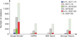
Modelling environments such as SIMSCAPE (MATLAB/SIMULINK) enable the creation of component blocks and their aggregation into higher-level thermal models for system analysis (MathWorks 2024), and have been explored by researchers such as Lapusan et al. (2016) and Mijlad et al. (2016). According to the authors’ own survey of academic publication repositories (Fig. 1), a growing interest has emerged in the scientific community in the use of such environments. Thermal modelling associated with SIMSCAPE is also exhibiting a vigorous trend over the last decade. Furthermore, using the keywords “therm,” “SIMSCAPE,” “black-box,” “gray-box,” and “white-box” in Google Scholar, 64 (2011-2015), 321 (2016-2020), and 952 (2021-2025) citations were found, thus showing a shared tendency.

Figure 1
History of citations related to keywords “SIMSCAPE” (S) and “therm*” (Th) (* = wildcard).

Despite these advances, no studies were found applying hierarchical thermal modelling methodologies to inertial navigation systems (INS) or inertial measurement units (IMU). Existing literature mainly focuses on system-level techniques such as thermal calibration and characterization (Wang et al. 2016), also aided by deep learning (Chen and Pan 2023) and error modelling (El-Sheimy and Youssef 2020). These approaches, however, do not include hierarchical integration from component to system level, which suggests a relevant opportunity for applying progressive, experimentally validated methodologies to INS/IMU systems.

The subsequent sections will provide a background on the primary concepts necessary for the decision-making process of the proposed M&I methodology, based on the four outlined steps. Once the M&I subject has been analyzed (or conceived), described, and associated with a specific-colored box (or boxes, if a hierarchical approach is adopted), the M&I procedure and its appropriate environments can be developed. Finally, the procedure will be applied to an INS, yielding theoretical and experimental results. The final section discusses the advantages of the proposed methodology.

METHODOLOGY

Overview

The first step of the M&I methodology, which precedes the selection of the box color, pertains to understanding the system being modelled and the intended purpose of the resulting model. This work focuses on an aerospace system that operates under demanding aerospace environmental conditions, specifically concerning thermal, vacuum, and humidity qualification ranges. Furthermore, (i) a system prototype is available, and (ii) measurements can be collected not only from the entire system but also from its individual components.

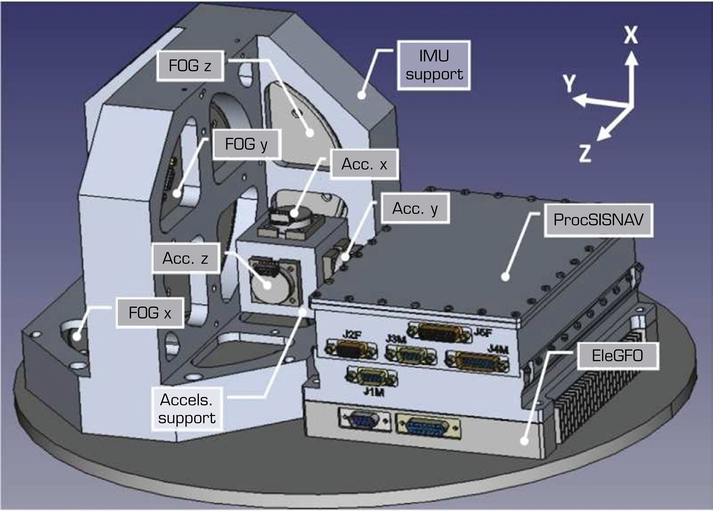
The subject of M&I will now be presented. The initial components of the INS designated as Sistema de Navegação Inercial (SISNAV) were conceived by the Brazilian Air Force (Força Aérea Brasileira) several years ago (Ramos 2015). This project aims to provide a national aerospace-grade INS for the governmental space program. Most of the critical components of SISNAV, such as the fiber-optic gyrometers (FOGs), the computer, and the voltage-to-frequency converters, were designed, produced, and qualified by both public and private organizations. The components of SISNAV are illustrated in Fig. 2, which does not include the current metallic case.

Figure 2
SISNAV components.

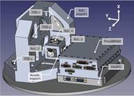
The following list identifies each SISNAV component:

• ProcSISNAV: SISNAV processor.

• EleGFO: power supply of the FOG triad.

• FOG_x, FOG_y, and FOG_z: FOG triad, each FOG mounted with respective axis orientation; these FOGs are also categorized in a later section as FOG_h and FOG_l (high and low angular rate, respectively).

• Acc_x, Acc_y, and Acc_z: accelerometer triad, each accelerometer mounted with respective axis orientation.

• Accelerometer support.

• IMU support.

• Metallic disk.

Colored box

Between the extreme white-box (pure theoretical modelling) and black-box (pure experimental modelling) approaches, real-world cases predominantly utilize mixed gray-box methods. These methods can be further classified into light-gray (physical laws with associated parameters expressed as differential equations) and dark-gray models (physical rules with unknown model structures and parameters represented by neuro-fuzzy models (Isermann and Münchhof 2010).

Consider a system comprised of known components, from which individual physical laws can be extracted. Additionally, some of these components may be substituted soon. In this context, physically modelling and identifying each component, followed by integrating these individual models – initially as submodels and subsequently as a unified set – represents an effective approach, ranging from white- to light-gray box modelling. Specifically, the replacement of a component necessitates the substitution of its corresponding model and, consequently, the retuning of its bonding parameters with respect to the remaining system.

The alternative to this approach could involve relying on an arbitrary model structure (either physically nonrepresentative or implicit) to be fed by experimental data, resembling a dark-gray to black-box approach. Consequently, for each component replacement, the entire M&I process must be repeated.

Consider a scenario in which one of the system components possesses a parametric set associated with time-variant, variable-dependent, nonlinear, or other specific behaviors (e.g., power consumption dependency on temperature). This behavior impacts the remaining components, such as the increase in temperature of a DC-DC power supply, which results in heat transfer to surrounding elements, and it may even feed back to the source component(s). These specific features can be effectively aggregated within the previously mentioned submodelled framework.

Parametrization

Finally, it is essential to examine the parameter set. Considering a system decomposed into its components, a valid approach involves modelling and identifying each component individually, subsequently building submodels and then tuning their respective interfacing parameters. Ultimately, the complete model is established, which enables the creation of a “macro model” that incorporates surrounding external components (e.g., the base plate and the fairing of the host vehicle), systems and/or environments (e.g., environmental qualification profiles), and scenarios (e.g., temperature variation due to the extended exposition to local weather conditions). It is also important to note that for physics-based models spanning a white-to light-gray box range, the parameters are typically known or require experimental tuning within their acceptable ranges.

The previous discussion was intentionally conducted towards light-gray physical modelling of a decomposed system, whose components were presented in the previous section. Consequently, the “intended use of the model” relies on its versatility for future component replacements and the associated simplicity of parameter retuning. This application will be clarified and illustrated in the subsequent sections. This discussion concludes the second step of the M&I methodology, namely, the selection of the box color.

The colored-box framework

The correlation of thermal model parameters with experimental data is a well-established practice in thermal engineering and SI. In this work, the intention is not to propose novelty in that procedure, but to situate the adopted methodology within the classical white-, gray-, and black-box framework, as discussed by Isermann and Münchhof (2010). This conceptual classification helps clarify the modelling philosophy adopted.

Physical modelling

The methodology progresses by selecting the theoretical and/or experimental setup for the execution of the M&I tasks. This decision must align with the objectives derived from the previously selected light-gray box. First, a well-defined model structure, incorporating physically representative components, must be established. Subsequently, the corresponding mathematical equations associated with a parametric setup can be formulated in various forms, including differential, state-space, transfer functions, or other appropriate forms.

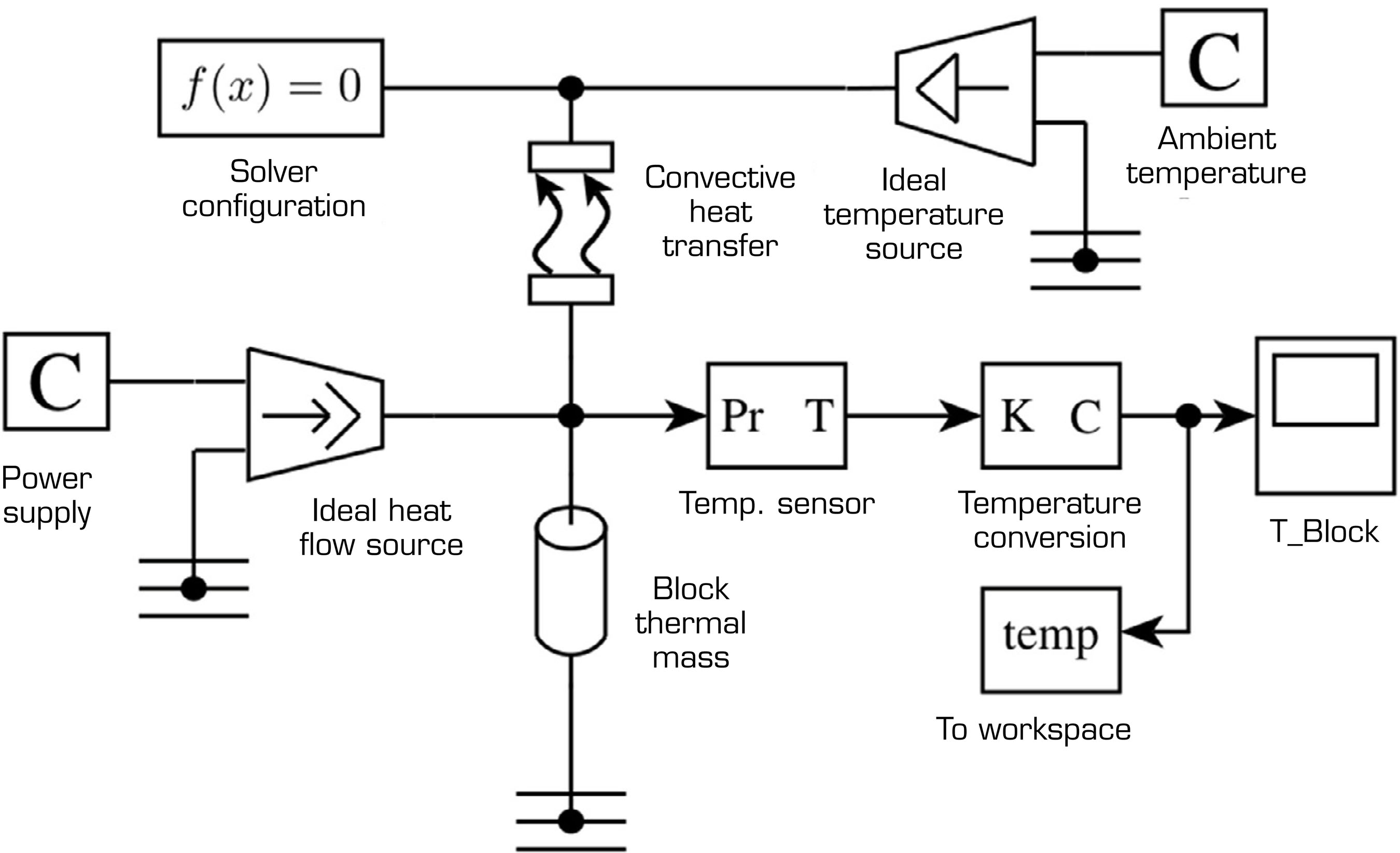
As an example, consider a metallic block heated by embedded resistors powered by the electric current from a power supply. Initially, it can be assumed that the heat distribution (and, consequently, the temperature) is homogeneous for those components with high thermal conductivity, such as the block itself. Furthermore, the block is supported by small spacers that act as thermal insulators, such that heat is transferred to the surroundings by convection only.

This configuration can be transcribed into a simulation model such as the one shown in Fig. 3. The elements of the simulation environment SIMSCAPE (MATLAB 2011) and the equivalent context in the thermal engineering theory (Lienhard and Lienhard 2024) are summarized in Table 1, where U is the internal thermodynamic energy (J), Q is the heat transfer rate (J s^-1 = W), C is the lumped thermal capacitance (J K^-1), ρ is the density (kg m^-3), c is the specific heat (J kg^-1 K^-1), V is the volume (m³), m is the mass (kg), L is the thickness in the direction of the heat flow (m), k is the thermal conductivity (W m^-1 K^-1), A is the area (m²), R_cond is the conductive thermal resistance (K W^-1), T_s is the surface temperature (K), T_amb is the ambient temperature (K), h is the heat transfer coefficient (HTC) (W m^-2 K^-1), R_conv is the convective thermal resistance (K W^-1), є is the emittance (–), σ is the Stefan-Boltzmann constant (5.67037 × 10^-8 W m^-2 K^-4), T_surr is the surroundings temperature (K), R_rad is the radiative thermal resistance (m^-2), Q_k (J s^-1), and T_k (K) are respectively the constant heat transfer rate and the constant temperature, and T_ref (K) is the reference temperature.

Figure 3
Thermal simulation model of a metallic block built with MATLAB’s SIMSCAPE.

Table 1
Characterization of thermal elements with classical (C) and SIMSCAPE (S) symbols.

Block	Definition	Symbols	Equations
Thermal mass	Lumped capacity that stores energy		Q = dU/dT = C dT/dt, where C = ρ c V = c m
Conductive Heat Transfer	Solid conduction between two nodes		Q = ΔT/Rcond, where Rcond = L/(kA)
Convective Heat Transfer	Convection from node to ambient		Q = (Ts - Tamb )/Rconv where Rconv = (hA)-1
Radiative Heat Transfer	Radiation between surface and surroundings		$Q=ϵ\sigma A(T_s^4-T_{\text{surr}}^4)\mid ,R_{\text{rad}}=(1-ϵ)/\left(ϵA\right)$
Ideal Heat Flow Source	Imposed heat rate		Q = Qk
Ideal Temperature Source	Imposed temperature boundary		T = Tk
Temperature Reference Point	Temperature reference to determine other ones		T ref

• Source: Elaborated by the authors.

Symbols used in the classic thermal theory are generally electric circuit analogues, e.g., heat transfer rate is equivalent to electric current (or Q ≡ I), and temperature to electric voltage (T ≡ V). In early releases (e.g., R2011a), conductive heat transfer was represented through material and geometric parameters using the “conductive heat transfer” block, being substituted by the “thermal resistance” block in newer releases. R_rad refers to the surface resistance in textbooks, while SIMSCAPE implements the full Stefan-Boltzmann equation directly. “Ideal temperature source” and “Ideal heat flow source” refer to the standard SIMSCAPE (MATLAB R2011a) boundary condition blocks; these blocks impose, respectively, a fixed temperature or a prescribed heat flow at a thermal node, regardless of the resulting energy required – they represent idealized, unlimited sources used to define thermal boundary conditions, not real heaters or dissipative devices. The “solver configuration block” defines numerical settings and reference parameters for the thermal network; it has no physical equivalent. The remaining elements are self-explicative: temperature reference point, temperature sensor, temperature conversion from Kelvin to Celsius, scope (“T_Block”), physical signal constant (“Ambient temperature” and “Power supply”), and sink block “To workspace” (“temp”).

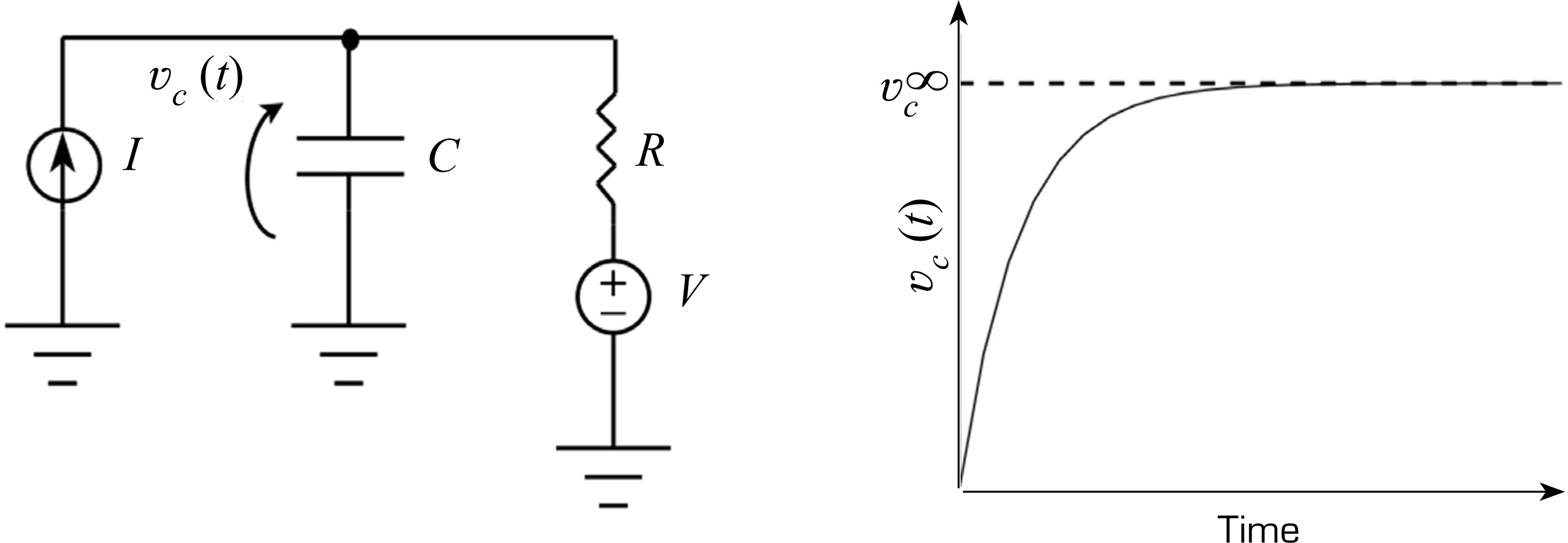
Figure 3 can be converted to other physical domains as the Fig. 4 electrical equivalent, where I (ampere) is an electric current source, C (farad) is a capacitor whose voltage is ʋ_c(t), R (ohm) is a resistor, and V (volt) is an electric voltage source.

Figure 4
Equivalent representation of the metallic block thermal model in the electric domain.

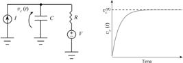
Using Kirchhoff’s current law, one finds Eq. 1, with steady state level ${\mathrm{v}}_{\mathrm{c}}^{\mathrm{\infty }}=\mathrm{V}+\mathrm{RI}$ and solution given by Eq. 2. From the respective graph in Fig. 4, one can note the exponential nature of the v_c(t) response (which is shared by the thermal analogue shown in Fig. 5 and Eq. 3, where T_m(t) is the metallic block temperature).

(1) $\frac{d{v}_c\left(t\right)}{dt}=-\frac{\left[v_c\right(t)-v_c^{\mathrm{\infty }}]}{RC},v_c^{\mathrm{\infty }}=V+RI$

(2) $v_c\left(t\right)=v_{\mathrm{\infty }}+(v_0-v_{\mathrm{\infty }})e^{-t/RC}\to v_0=0\to v_c\left(t\right)=v_{\mathrm{\infty }}(1-e^{-t/RC})$

Figure 5
Thermal model of the metallic block.

(3) $\begin{array}{c}\frac{d{T}_m\left(t\right)}{dt}=-\frac{\left[T_m\right(t)-T_m^{\mathrm{\infty }}]}{R_{conv}{C}_m}\\ T_m^{\mathrm{\infty }}=T_k+R_{conv}{Q}_k\\ T_m\left(t\right)=T_m^{\mathrm{\infty }}(1-e^{-t/R_{conv}{C}_m})\end{array}$

Given that the principles of model structuring have been defined, along with the required components and their respective equations, one can now proceed to establish theoretical and experimental environments.

Simulation and experimental environments

Simulation environment

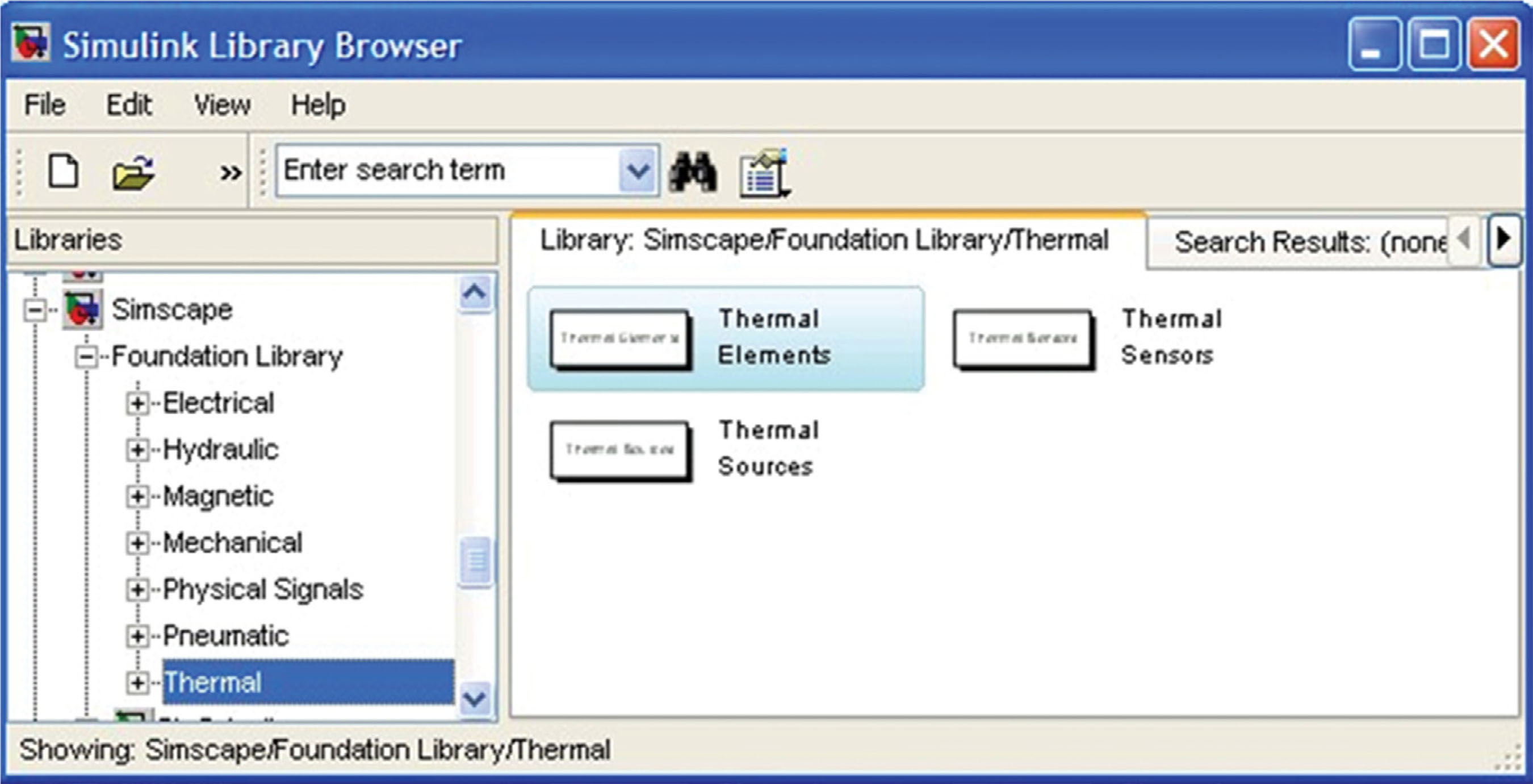
To create the thermal models that are utilized in this study, along with their components, one employs MATLAB and SIMULINK version 7.12 (R2011a) (MATLAB 2011) or, more precisely, SIMSCAPE (a software extension with tools for modelling and simulating multi-domain physical systems) with its thermal foundation library (Fig. 6).

Figure 6
The main SIMULINK library used in this work.

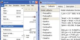
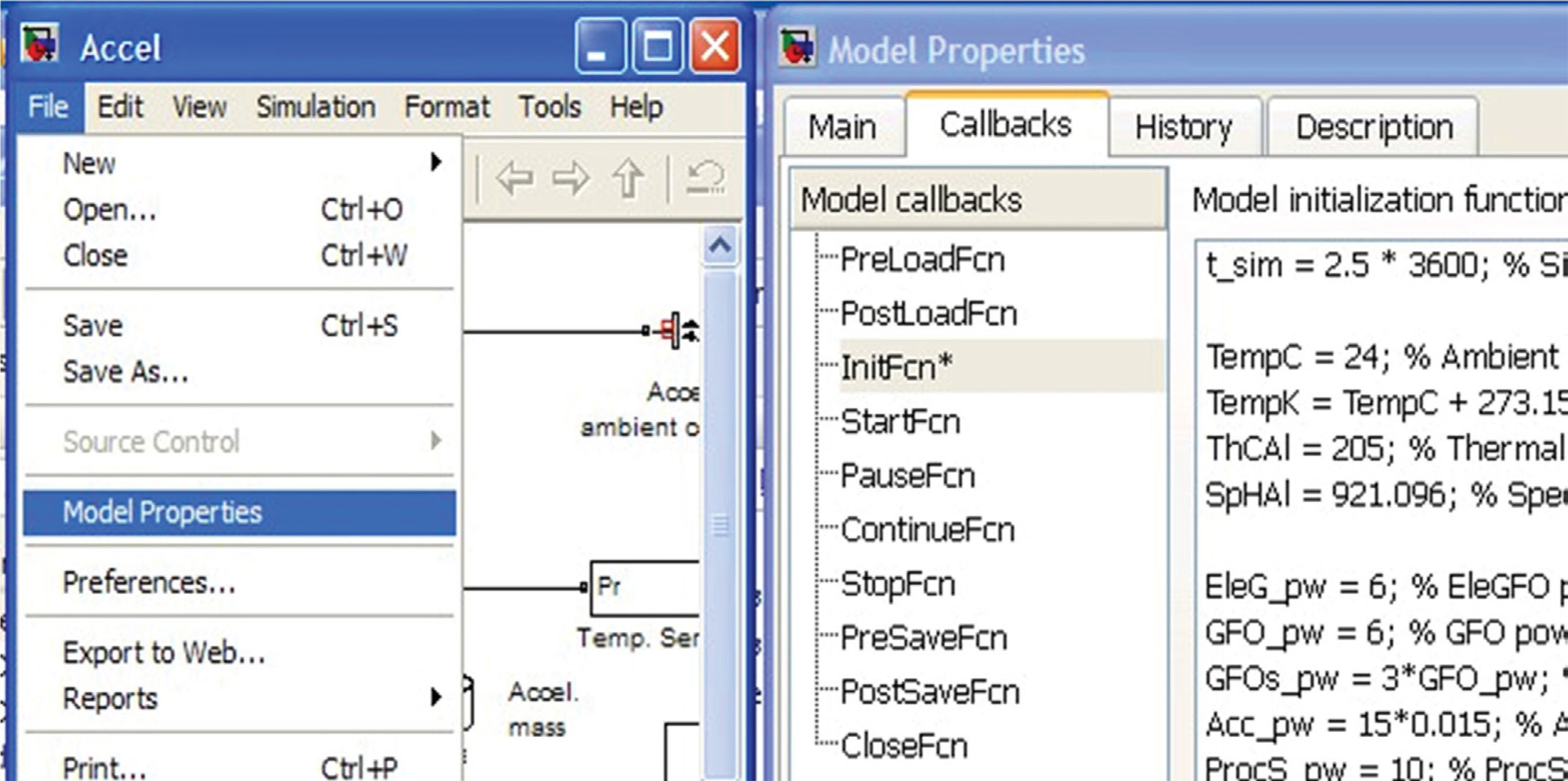
To construct a new model, one selects the option “File => New => Model” from the MATLAB pop-up menu. Subsequently, simulation blocks can be inserted and connected. These blocks require numeric values, such as parameters and conversion factors, which must be defined in advance. This task is facilitated if these parameters are stored in the InitFcn model callback, located under the “Callbacks” tab in the “Model Properties” menu of the simulation file window (Fig. 7).

Figure 7
Tab InitFcn tab of the simulation model properties.

Experimental environment

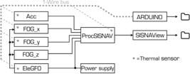
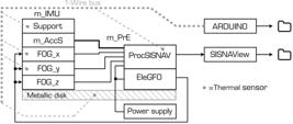
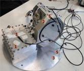
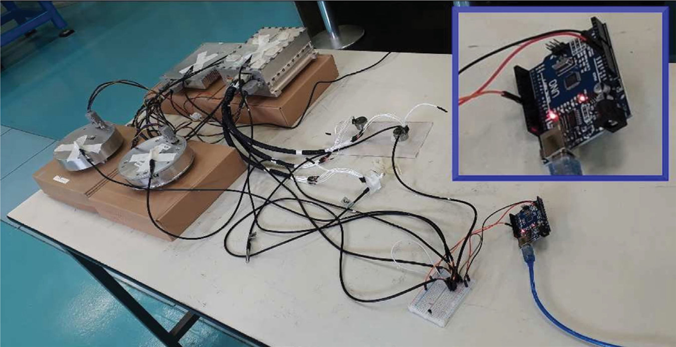
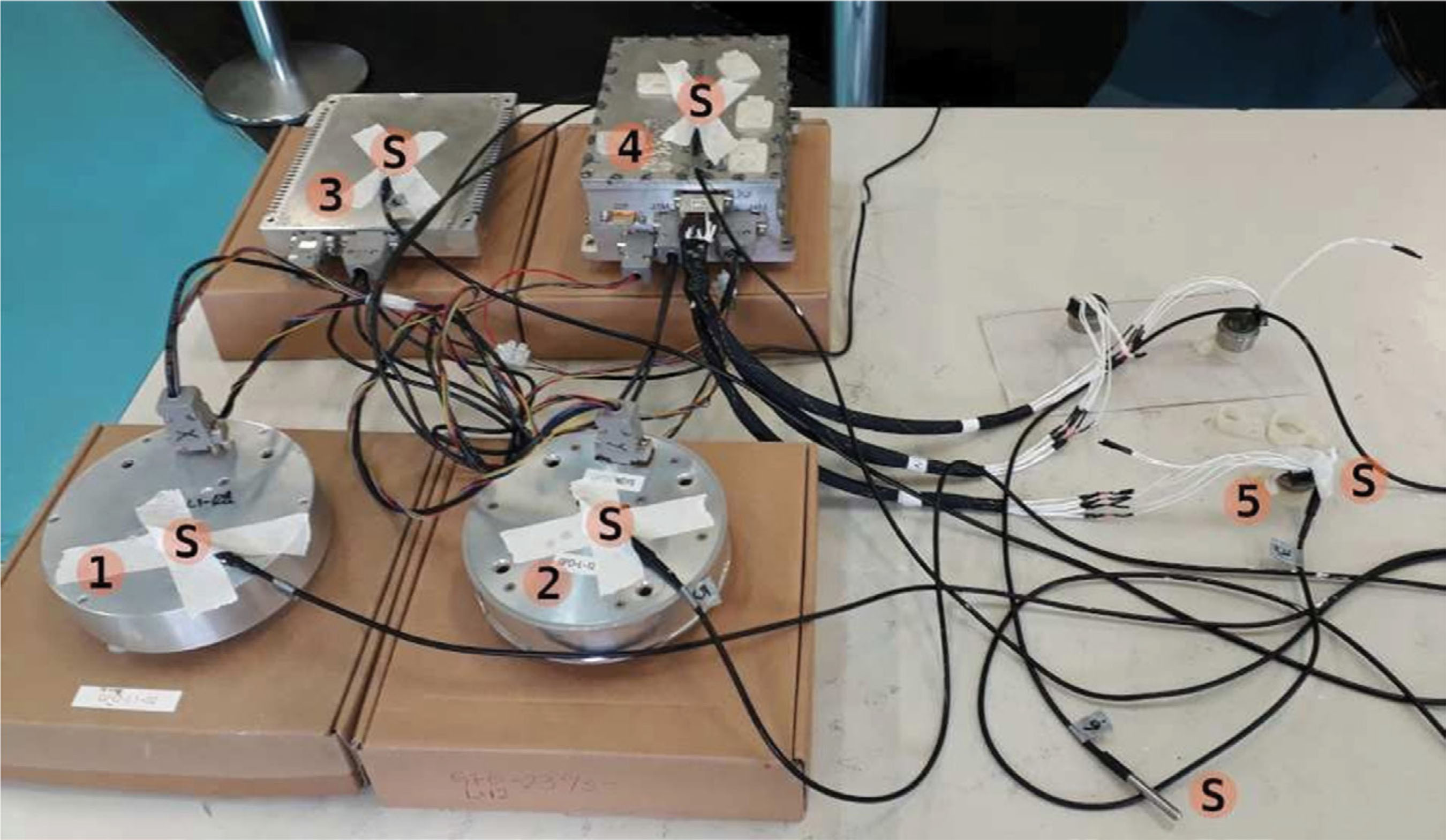
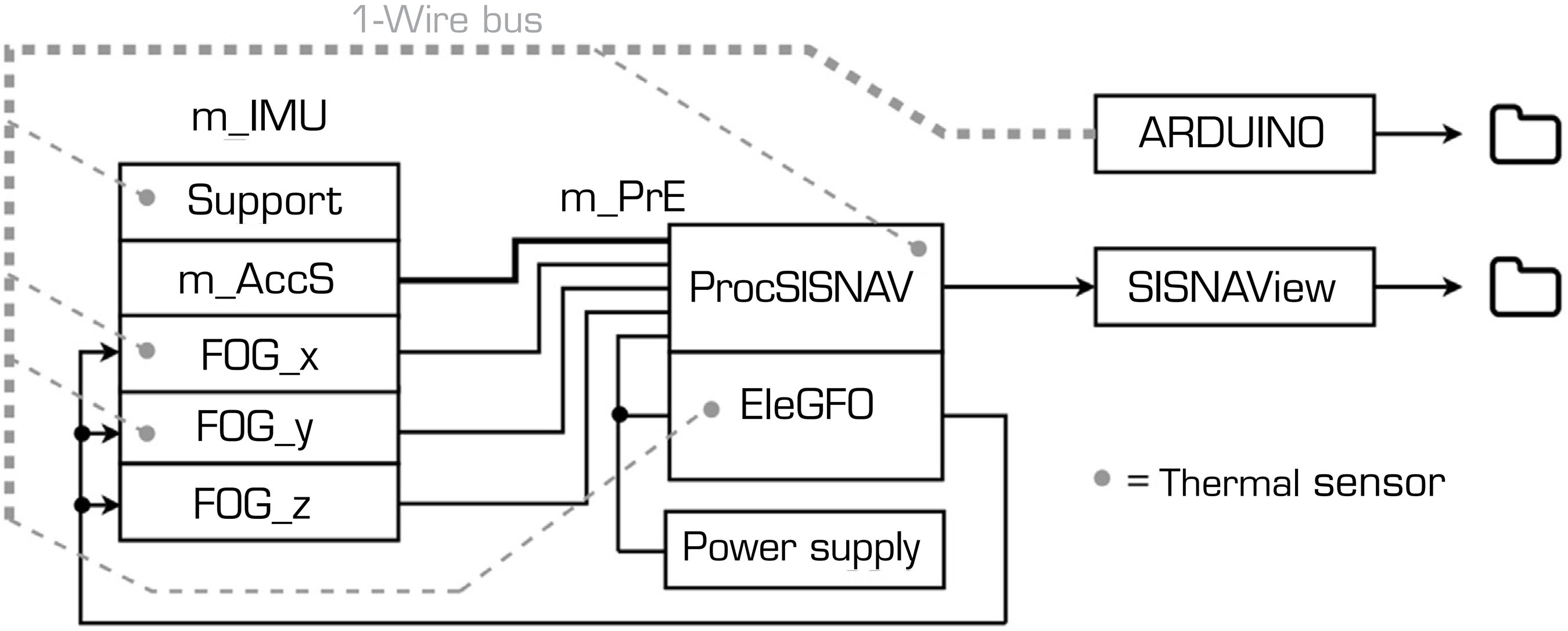
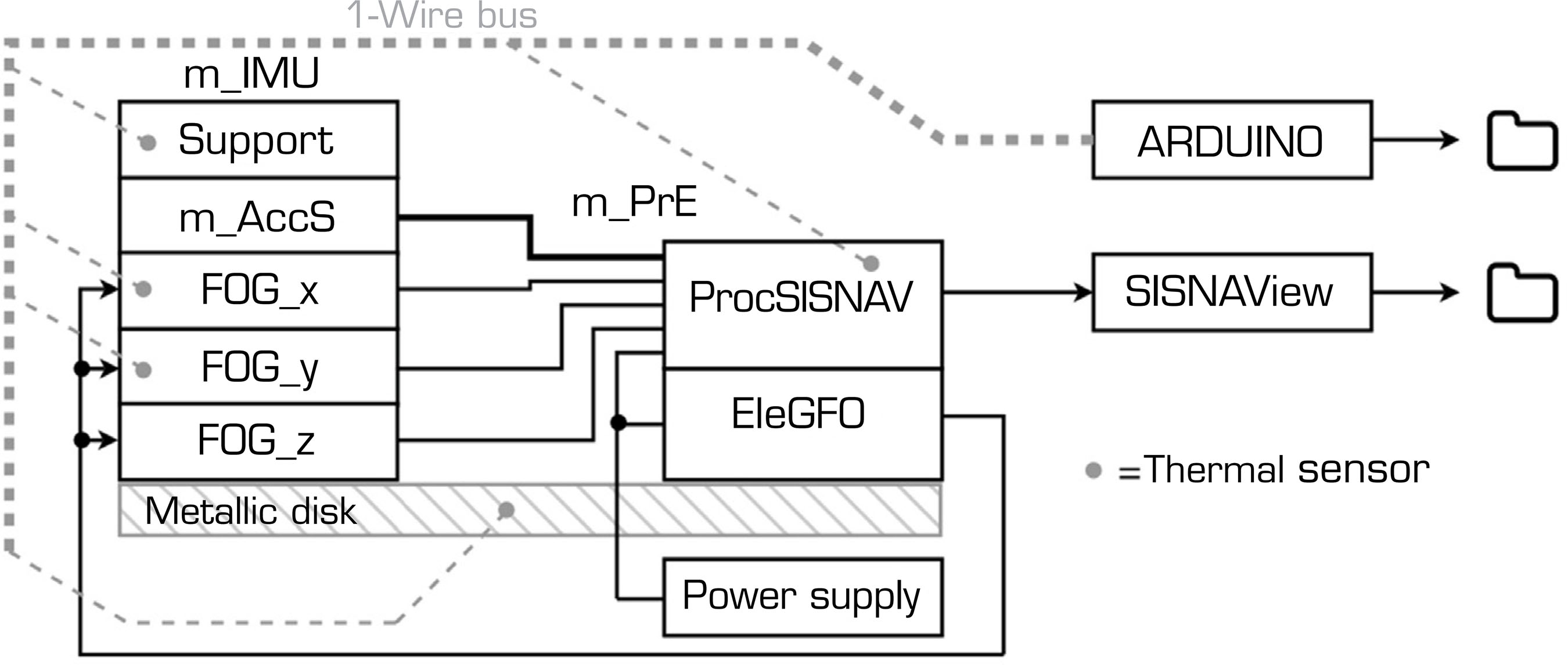
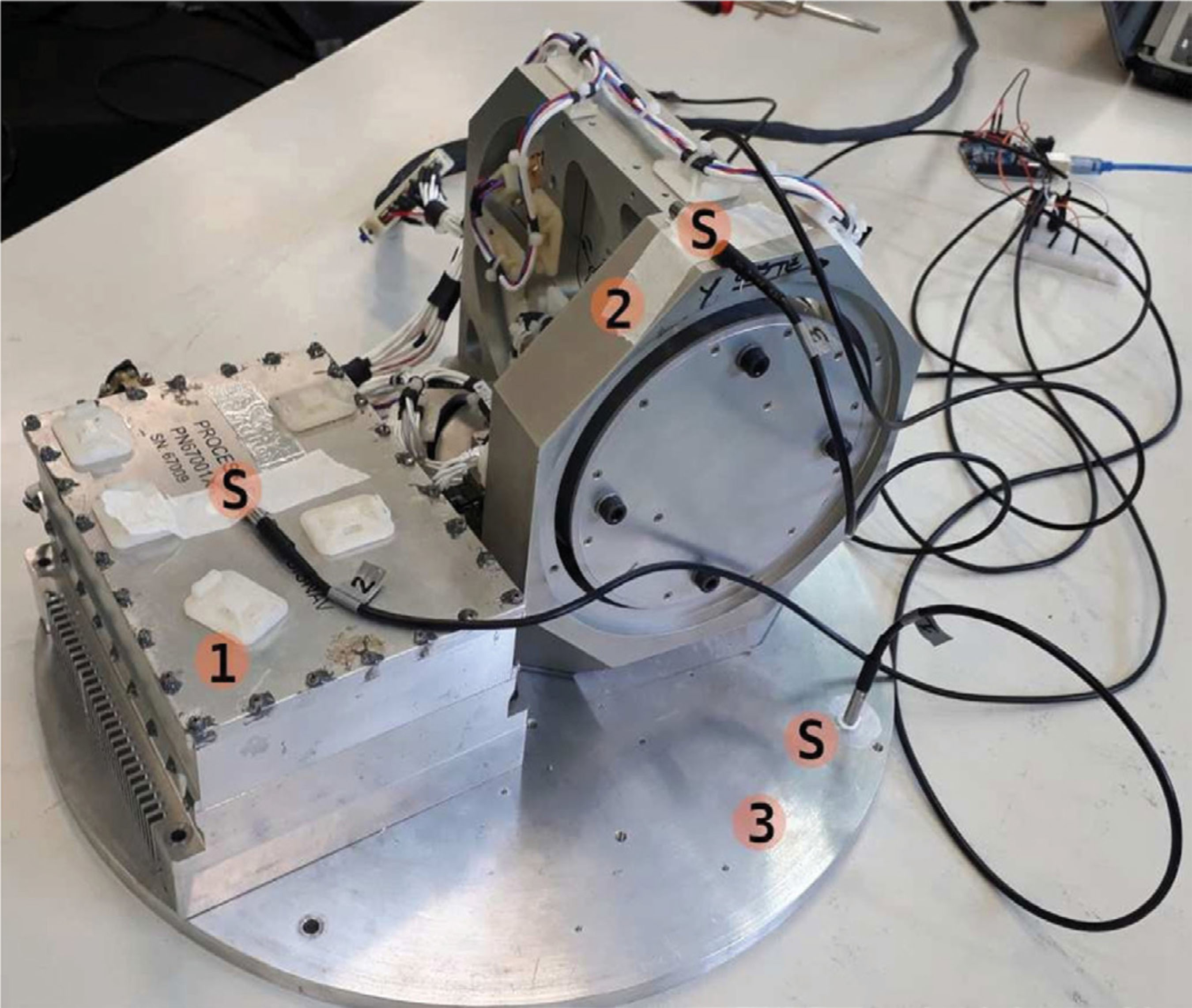
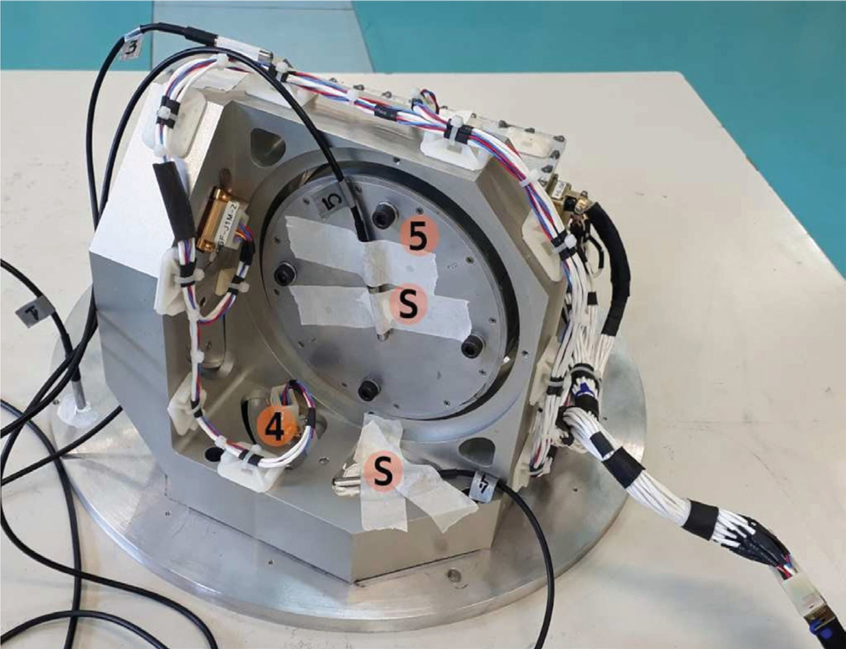
Experimental setups were devised for components (Figs. 8-10), submodels (Fig. 11), and the full SISNAV model (Figs. 12-14). A power supply is connected to ProcSISNAV and EleGFO; the power output of the latter is connected to the FOGs. Arduino thermal sensors are fixed to each of the selected SISNAV components.

Figure 8
Experimental setup for SISNAV components.

Figure 9
Arduino board with temperature sensors fixed on non-aggregated SISNAV components.

Figure 10
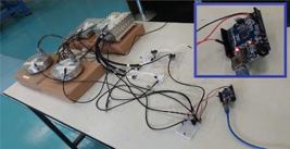
Identification of the non-aggregated experiment elements. Labels indicate: 1-2 = high- and low-angular-rate fiber optic gyroscopes; 3 = EleGFO; 4 = ProcSISNAV; 5 = accelerometer; S = thermal sensors. The bottom-right thermal sensor measures ambient temperature.

Figure 11
Experimental setup for SISNAV submodels.

Figure 12
Experimental setup for SISNAV full model with metallic disk.

Figure 13
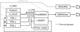
Identification of the fully aggregated experiment elements. Labels indicate: 1-2 = high- and low-angular-rate fiber optic gyroscopes; 3 = EleGFO; S = thermal sensors.

Figure 14
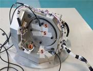
Identification of the fully aggregated experiment elements. Labels indicate: 4 = ProcSISNAV; 5 = accelerometer; S = thermal sensors.

ProcSISNAV interfacing comprises RS-422 ports to the FOGs and analogue signal lines to the accelerometers. ProcSISNAV sends data packets to SISNAView, a National Instruments/LabVIEW application. Arduino’s and SISNAView’s acquired data are then stored in digital files for post-processing.

The parameter optimization of each component, submodel, and the entire system is achieved from temperature measurements obtained from them. The ambient temperature of the host laboratory will also be recorded to verify whether external disturbances are negligible.

Measurements

Thermal measurements (“S” signs shown in Figs. 10, 13, and 14) of SISNAV components were recorded with Arduino (Fig. 9), an open-source electronics platform (The Arduino Team 2024).

Thermal sensor specifications (Arduino) – DS18B20 (manufacturer: MAXIM, formerly Dallas Semiconductors): temperature range: -55 to +125 ^oC; accuracy: ± 0.5 ^oC (-10 to +85 ^oC); resolution: 9 to 12 bits (programmable); 1-Wire bus; single-point calibration performed at 0 ^oC (ice water mixture) for all sensors.

Thermal sensor specifications (ProcSISNAV) – The temperature measurement of each accelerometer is based on the current of its internal electrical source. On the SISNAV/ProcSISNAV side, this current produces a dropout voltage on a precision resistor, which is digitized by an analog-to-digital converter, yielding an absolute error of ± 3.0 ^oC for the temperature range of -55 to +96 ^oC.

• Applied torques to fix the components: screws fixed by hand (not using a tool).

• Cleaning: performed only at the interface and sensor surfaces.

• Thermal grease: applied to the temperature sensors only.

A procedure for system M&I – The third step of the M&I pertains to the adopted procedure for model building, evaluation, and validation. In this aggregated case, the following progressive actions are proposed:

• Develop and construct the thermal model for each component;

• Calibrate each model’s parameters using measured data;

• Create submodels of components by integrating the previously developed models;

• Adjust the additional (interfacing) parameters of the submodels based on measured data;

• Combine all submodels to obtain the complete thermal model (full model);

• Tune the additional parameters of the full model using measured data;

• Simulate the full model according to scenarios related to specified (or required) environmental conditions, such as temperature, humidity, and vacuum;

• Conduct laboratory tests on the full real model under the previously defined environmental conditions, comparing the results of the simulations with the test outcomes;

• Create a macro model composed of the full model and its host system;

• Calibrate it with measured data or assign appropriate values to the new parameters;

• Run the macro model in accordance with the host scenarios;

• Design and implement a validation program for the macro model, which includes environmental tests and an experiment conducted on board the host system.

Humidity

Classical heat transfer equations do not contain humidity directly because they model only heat. However, humidity environmental tests are useful to evaluate the unmodelled effects of changing material properties (humid air versus dry air) or evaporation/condensation latent heat and mass transfer terms. Such effects are worth exploring in future work.

Vacuum

Under very low-pressure conditions, convective HTCs were assigned negligible values (≈ 0 W m^-2 K) to represent the absence of gaseous conduction. Consequently, heat exchange between components was modelled exclusively through solid conduction. Thermal contact resistances at mechanical interfaces were not explicitly represented in the present model. Accordingly, the resulting temperature predictions are intended for qualitative interpretation, emphasizing relative temperature distributions and temporal trends rather than absolute temperature values.

Simplifying assumptions

This study aims to develop a preliminary thermal model of SISNAV to establish a baseline expectation of its behavior under specific environmental conditions. Consequently, it is essential to consider some restrictive assumptions:

Composition

Each SISNAV component comprises a mixture of materials, some of which are not effective thermal conductors (e.g., the glass fiber in printed circuit boards (PCBs). Instead of evaluating each of these components in detail, one aims to develop a truncated model, focusing on the predominant material (e.g., the metallic case); its physical characteristics are taken as the first guesses of the model parameters. This modelling is known as “lumped capacitance” (Incropera 2006) and is a reliable and simplified approach when a set of components must be analyzed simultaneously. The main hypothesis is that the components have uniform temperature. The accuracy of this approach depends on the Biot number of the element (Bi = hLK^-1, where h is the convection heat transfer coefficient, L is the characteristic length, and k is the thermal conductivity). When Bi << 1 (which is the case in this work), accuracy rises. Furthermore, the models’ parameters are posteriorly tuned according to the experimental data.

Parameter tuning

The models’ parameters are manually tuned for error minimization between the simulation outputs and the real measurements obtained from experiments conducted with the component, submodel, or system. Consequently, it is evident that establishing a series of progressive steps is essential for the gradual tuning of the parameters for each component or submodel.

Performing the M&I Procedure

Regarding the M&I procedure, the thermal models to be developed and calibrated are presented in the following list (note that this list does not fully comply with the adopted procedure for model building of the M&I methodology; the remaining actions will be addressed in future work):

• Accelerometer model Acc, incorporating convective thermal transfer only;

• Two FOG models (FOG_h and FOG_l), each incorporating convective thermal transfer only;

• FOG’s power supply model (EleGFO), incorporating convective thermal transfer only;

• Processor model (ProcSISNAV), incorporating convective thermal transfer only;

• Submodel m_PrE, which includes ProcSISNAV and EleGFO;

• Submodel m_AccS, comprising three accelerometers with the respective support;

• Submodel m_IMU, consisting of a triad of FOGs, m_AccS, and the IMU support;

• SISNAV thermal model (Sd), composed of the submodels m_PrE and m_IMU mounted on a metallic disk.

Nomenclature

Components of submodels can be identified by suffixes added to the submodel names. Example: m_IMU_FOGl addresses the component FOG_l of the submodel m_IMU. Aliases of the given components’ and submodels’ names are used eventually for the sake of shortening labels (examples: PrS instead of ProcSISNAV; PrE instead of ProcSISNAV + EleGFO), being contextually interpreted.

It is relatively straightforward to tune the parameters of a well-known component (e.g., the metallic block with embedded resistors mentioned in section “Physical Modelling”). However, the SISNAV components do not conform to this case, as most of them consist of multiple, not perfectly characterized internal components. This presents an additional rationale for employing simplified and aggregation-based modelling techniques, as well as for tuning the internal and interfacing parameters based on the correlation between simulation results and corresponding laboratory measurements.

SETUPS, RESULTS, AND DISCUSSION

As mentioned earlier, the full SISNAV thermal model is decomposed first into components, which are subsequently aggregated as submodels. Figure 3 shows the simulation model chosen for all components, which will be combined further as submodels. “Block mass” and “Power supply” parameters are set, respectively, with each of the Acc_x/y/z, FOG_x/y/z, EleGFO, and ProcSISNAV components’ masses and electric power values. The remaining block (“convective heat transfer“) is the same, but with the respective parameters. The housings of most components are made of 7075 aluminium, except for the accelerometer (steel).

SIMSCAPE blocks require input parameters, as identified in the following list. The InitFcn function of each block contains all definitions and/or computations of these parameters:

• Conductive heat transfer: area, thickness, and thermal conductivity;

• Convective heat transfer: area and HTC;

• Mass: mass, specific heat, and initial temperature;

• Physical signal constant: constant (assigned as ambient temperature or power).

Accelerometer thermal model

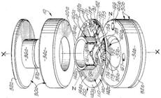
This component is an off-the-shelf product. While complete knowledge of its internal structure is lacking, some insights were gained by examining the documentation of a similar patented accelerometer (Fig. 15), which appears to align with the manufacturer’s description of the SISNAV component: “The accelerometer consists of two main subassemblies: a pendulous mass with integral flexures and capacitive translatory transducer, which is forced to balance by electromagnetic torquer, in a hermetically sealed package, driven by a servo loop electronic circuit” (reference not given for confidentiality restrictions).

Figure 15
Exploded view of the accelerometer described in U.S. Patent No. 3,702,073.

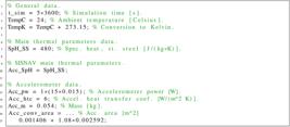
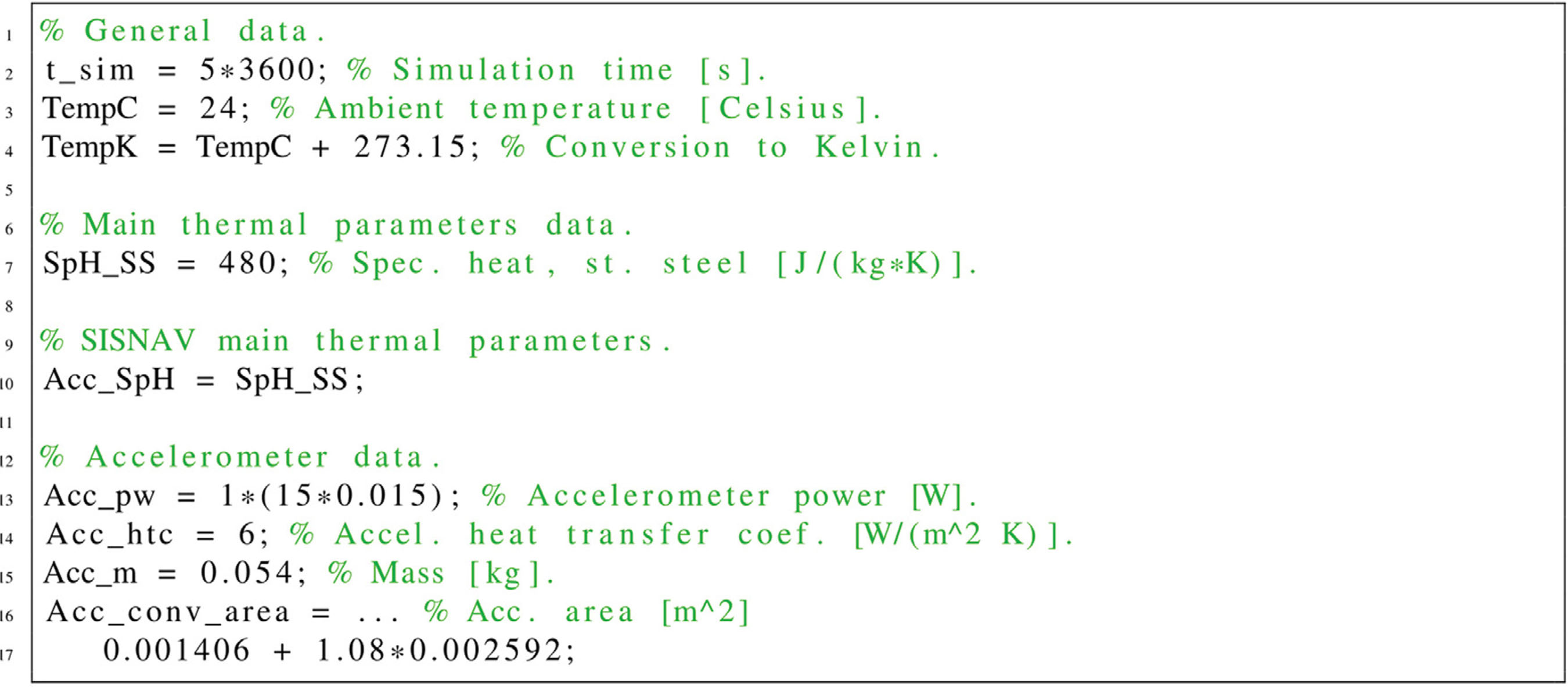
The contents of the InitFcn of the accelerometer thermal simulation model (equivalent to Fig. 3) were replaced with the script presented in Fig. 16. A computer-aided design (CAD) model was developed for the accelerometer to compute its total convective area. This area will be divided into conductive and convective portions when constructing the m_AccS submodel (the same reasoning applies to the other submodels).

Figure 16
Contents of the accelerometer model InitFcn function.

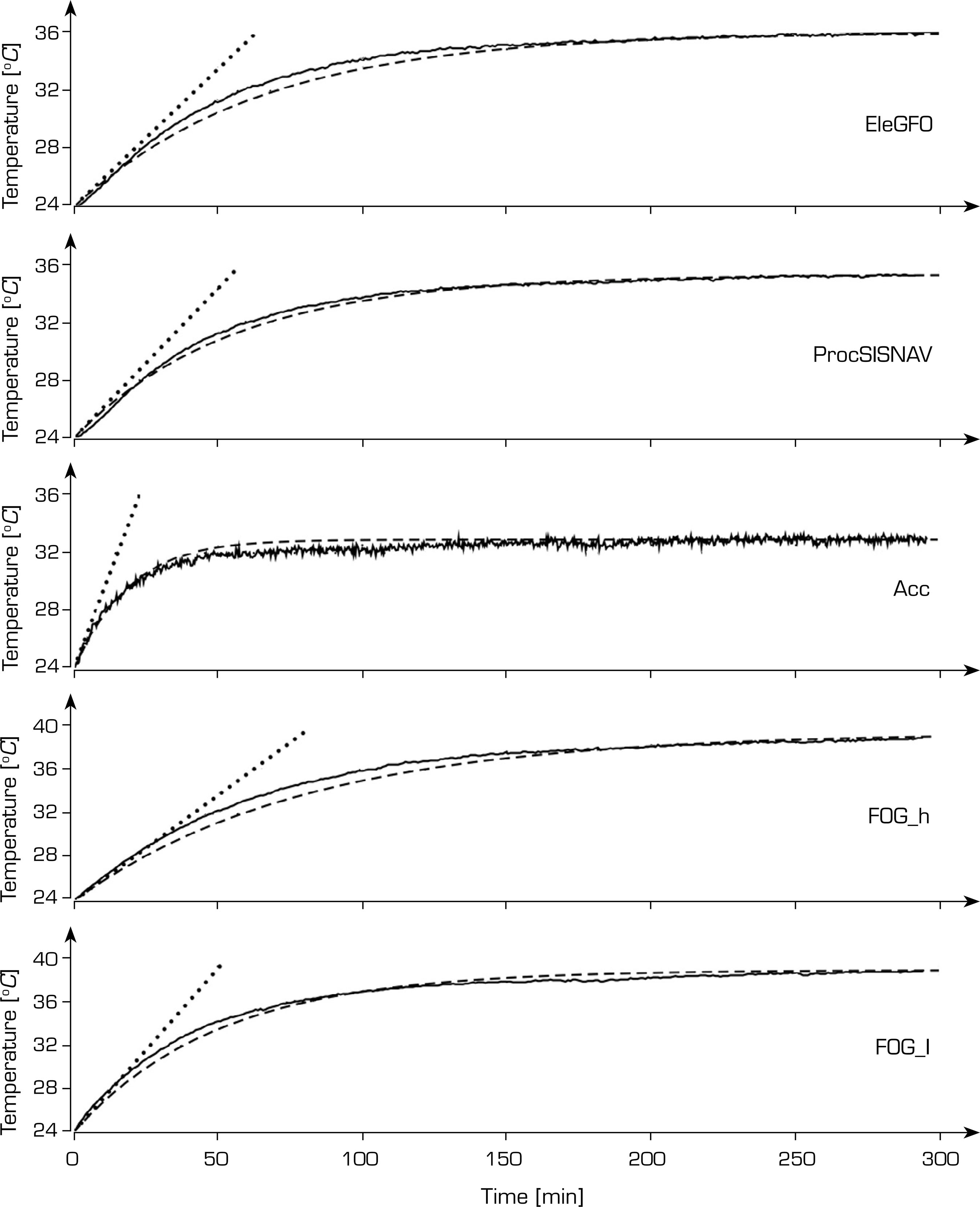
After fine-tuning the parameter “convective area,” a reasonable match was achieved between the experimental and simulation results, as shown in Fig. 17. For an HTC value of 6 W m^-2 K^-1, the temperature reached a steady state after approximately 4 hours, with an increase of around 9 ^oC. The maximum variation of the ambient temperature was 0.7 ^oC. The model behavior under vacuum conditions (HTC ≈ 0 W m^-2 K^-1) associated with qualification environmental tests is also shown.

Convective area adjustment

The aggregation of the thermal sensor and accelerometer cases with thermal grease was relevant in changing the interfacial resistance, slightly increasing the effective convective area of the assembly (not the geometric one, which is fixed).

Model behavior under vacuum

The linear rise for HTC ≈ 0 W m^-2 K^-1 results from pure internal heat generation and negligible external heat loss, that is, R_conv≈0 in Eq. 3. When convection is included, the curve asymptotically approaches a steady-state value through exponential evolution. Thus, convection establishes an equilibrium between generated and dissipated heat, acting as the dominant mechanism for thermal control of the device.

Accelerometer noisy measurement

The Arduino thermal sensor area is relevant in comparison with the accelerometers, which could affect the accuracy of the measurement. Therefore, the Arduino measurements were substituted with the ProcSISNAV ones, sampled at a higher rate, and filtered.

FOG thermal models

There are two FOG versions: low angular rate (used for the Y and Z axes) and high angular rate (for the X axis). Consequently, individual CAD and thermal models were developed for each version.

The maximum power consumption for both FOG versions is 6 W. However, this consumption primarily depends on the temperature stabilization circuitry associated with the laser emitter, whose behavior is unknown. A constant power value was tuned in the model to best align simulated and experimental results.

Figure 17 presents the simulations of the FOG models. For FOG_l HTC = 5 W m^-2 K^-1, the temperature reaches steady state in approximately 5 hours – faster than the high-rate model due to its smaller mass – with a temperature increase around 15 ^oC (same for both models). The adjusted HTC for FOG_h was 4.8 W m^-2 K^-1.

Figure 17
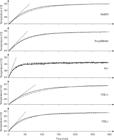
Comparison between thermal simulation results and experimental data for non-aggregated components. Continuous line = measurement; dashed = simulated; dotted = simulated (HTCs ≈ 0 W m-2 K-1).

ProcSISNAV thermal model

The maximum power consumption for the ProcSISNAV is 6.8 W. Figure 17 presents the simulation of its thermal model. For an HTC = 6 W m^-2 K^-1, the temperature achieves steady state in approximately 5 hours, with a temperature increase of around 11 ^oC.

EleGFO thermal model

EleGFO is simply a box with an EMI/EMC filter and a DC-DC converter, required to supply +5 V to the FOGs at a given power efficiency. Figure 17 presents the simulation of its thermal model. For an HTC = 2.2 W m^-2 K^-1, the temperature achieves steady state in approximately 5 hours, with a temperature increase of around 12 ^oC.

HTC values

The converter and filter are mounted on a PCB, inside the metallic housing of the EleGFO. This configuration qualitatively explains the low value adjusted for the HTC parameter of the simulation model (see also the discussion in the section “Theoretical/effective HTC”). Now, for the FOG_l case, its power consumption is not necessarily constant but depends on the internal thermal control. Conversely, the SIMSCAPE “Convective heat transfer” block assumes a constant HTC value. As part of the FOG’s power generates heat, so the variation of the former indirectly impacts the HTC. Even so, the SIMSCAPE block was adjusted to best match the simulation and experimental plots.

Submodels

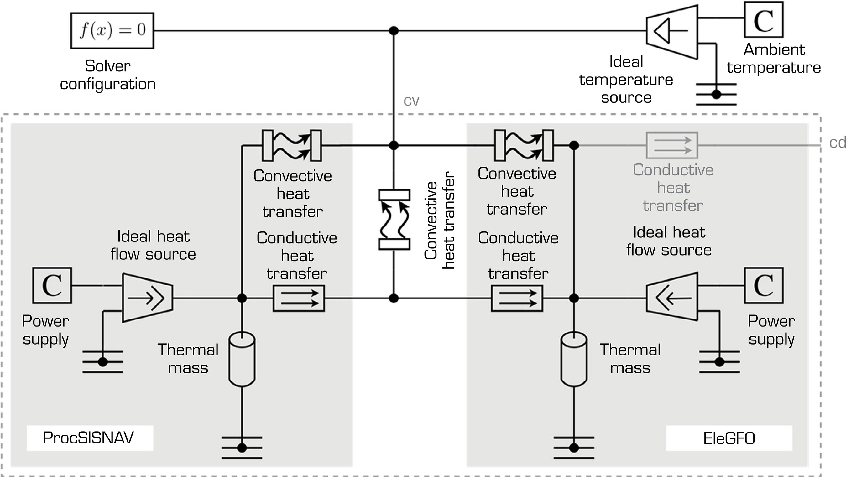
The submodel m_PrE consists of ProcSISNAV and EleGFO components, stacked one on top of another. Its simulation model is presented in Fig. 18. Conductive heat transfer blocks were added to their previous thermal models to represent the thermal exchanges between these subsystems. Consequently, the original convective-only areas of both components were divided into convective and conductive fractions. Note also the ports “cd” and “cv,” which are used in higher hierarchical levels, and are also applicable to the other submodels.

Figure 18
Thermal simulation submodel m_PrE.

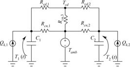
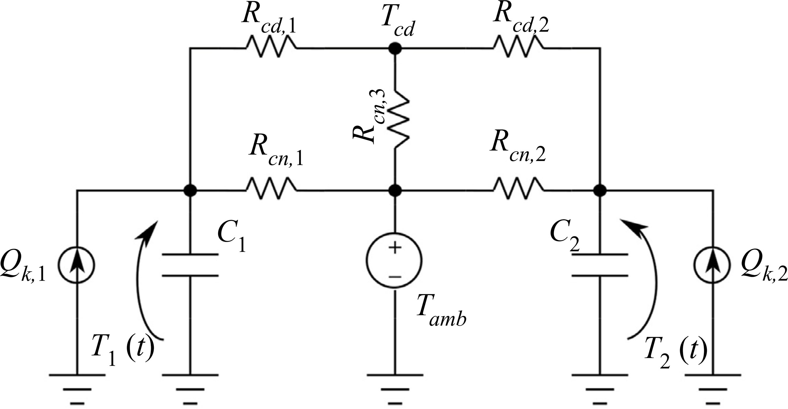
The respective thermal diagram of this submodel is presented in Fig. 19, where T₁(t) and T₂(t) are the temperatures of the thermal masses C₁ and C₂, R_cn,1, R_cn,2 and R_cn,3 are convective thermal resistances, R_cd,1 and R_cd,2 are conductive thermal resistances, Q_k,1 and Q_k,2 are heat flow sources, and T_amb is a temperature source. One can note the presence of an element between nodes T_cd and T_amb. This additional convective resistance R_cn,3 was included to represent minor heat losses through small air gaps that typically arise when two modules are simply stacked without mechanical fastening. In configurations where the contact pressure is increased, such as when screws or thermal paste are applied, these gaps are effectively eliminated, suppressing the associated convective path. Under these conditions, R_cn,3 becomes physically negligible and can be omitted from the thermal representation.

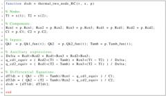
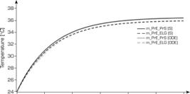
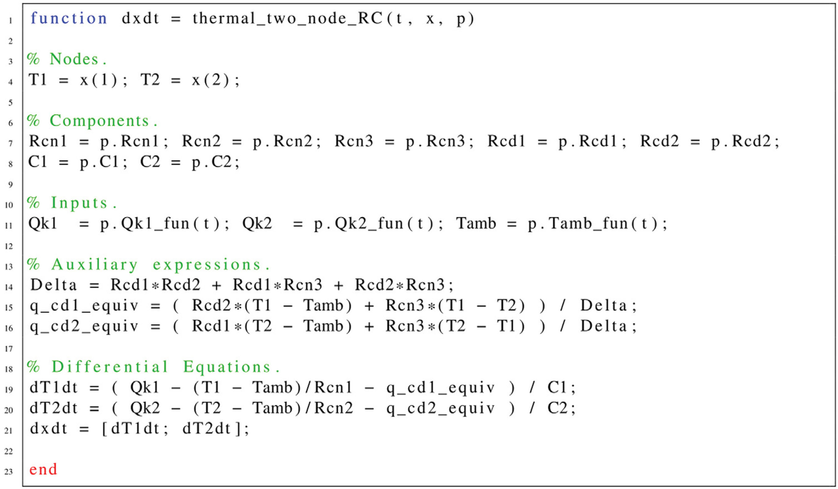
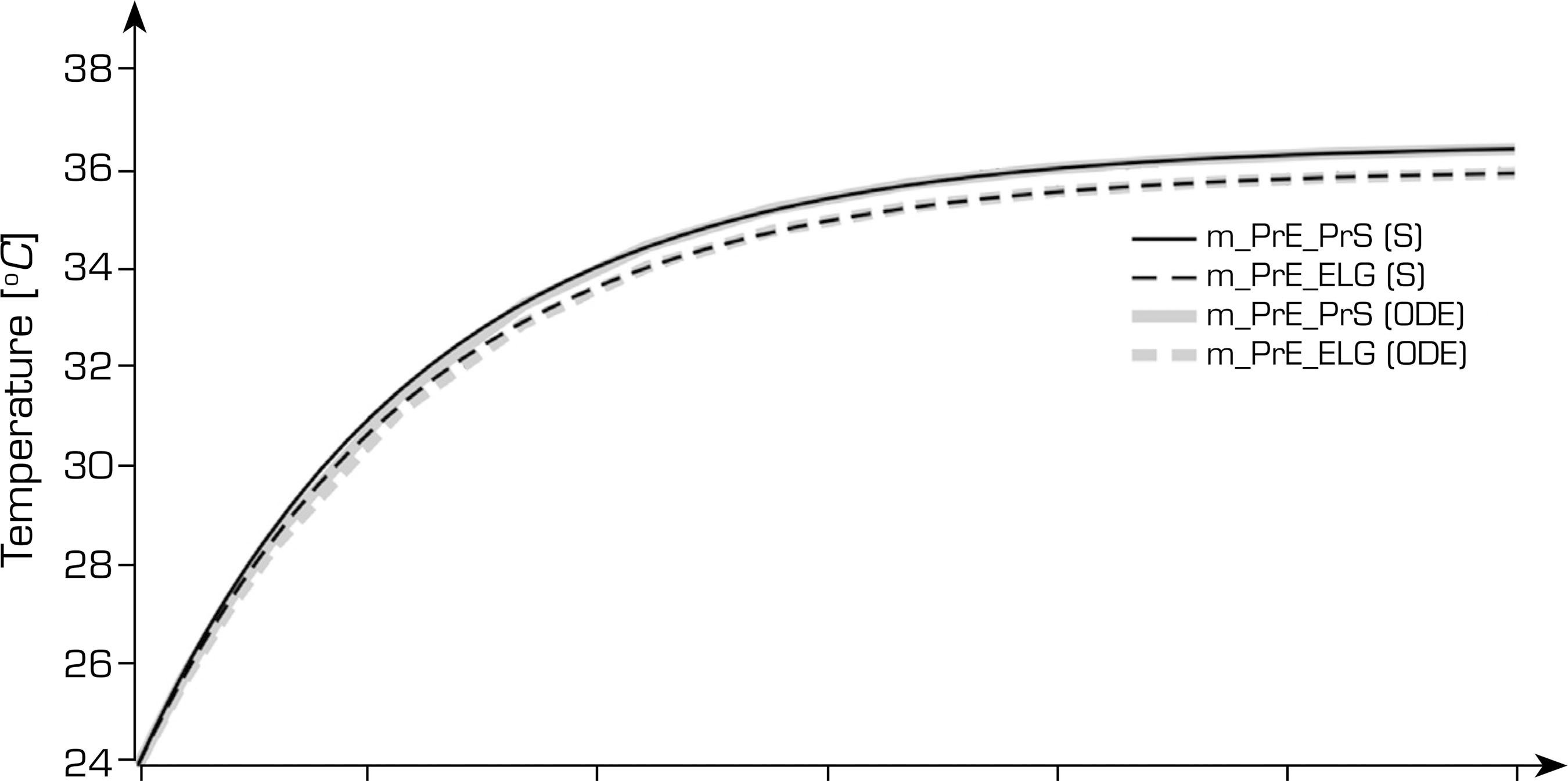
The mathematical representation of Fig. 19 is given by Eq. 4, which was translated into a MATLAB function (Fig. 20) containing the set of ordinary differential equations (ODEs). This function is called by another script, which feeds input parameters and sets the ode15s integration method, identical to SIMSCAPE’s. The comparison between SIMSCAPE and ODE results is presented in Fig. 21.

Figure 19
Thermal submodel m_PrE.

Figure 20
MATLAB ODE used to validate the submodel m_PrE simulation model.

Figure 21
Comparison between SIMSCAPE and ODE results for submodel m_PrE components.

(4) $\begin{array}{rl}{C}_1\frac{d{T}_1\left(t\right)}{dt}=& Q_{k,1}-\frac{\left[T_1\right(t)-T_{amb}]}{R_{\mathrm{cn},1}}\\ & -\frac{\{R_{\mathrm{cd},2}\left[T_1\right(t)-T_{amb}]+R_{\mathrm{cn}3}\left[T_1\right(t)-T_2(t\left)\right]\}}{\mathrm{\Delta }}\\ C_2\frac{d{T}_2\left(t\right)}{dt}=& Q_{k,2}-\frac{\left[T_2\right(t)-T_{amb}]}{R_{\mathrm{cn},2}}\\ & -\frac{\{R_{\mathrm{cd},1}\left[T_2\right(t)-T_{amb}]+R_{\mathrm{cn}3}\left[T_2\right(t)-T_1(t\left)\right]\}}{\mathrm{\Delta }}\end{array}$

with $\mathrm{\Delta }=R_{cd,1}{R}_{cd,2}+R_{cd,1}{R}_{cn,3}+R_{cd,2}{R}_{cn,3}$

Equation 4 can also be expressed in matrix form (Eq. 5). The corresponding solution, Eq. 6, has c₁ and c₂ determined by the initial conditions T(0) = [T₁(0) T₂(0)]^T , being the pairs {λ₁ λ₂} and {v₁ v₂} as a matrix’s eigenvalues and vectors, respectively.

(5) $\begin{array}{rl}& \dot{\mathit{T}}\left(t\right)=\mathit{A}\mathit{T}\left(t\right)+\mathit{b},where\left[\begin{array}{c}{T}_1\left(t\right)\\ T_2\left(t\right)\end{array}\right],\mathit{A}=\left[\begin{array}{ll}{a}_{11}& a_{12}\\ a_{21}& a_{22}\end{array}\right],\mathit{b}=\left[\begin{array}{c}{b}_1\\ b_2\end{array}\right],with\\ & \begin{array}{rl}{a}_{11}=& -\frac{1}{C_1}(\frac{R_{\mathrm{cd},2}+R_{\mathrm{cn},3}}{\mathrm{\Delta }}+\frac{1}{R_{\mathrm{cn},1}}),a_{12}=\frac{1}{C_1}\left(\frac{R_{cn,3}}{\mathrm{\Delta }}\right)\\ a_{21}=& \frac{1}{C_2}\left(\frac{R_{cn,3}}{\mathrm{\Delta }}\right),a_{22}=-\frac{1}{C_2}(\frac{R_{\mathrm{cd},1}+R_{\mathrm{cn},3}}{\mathrm{\Delta }}+\frac{1}{R_{\mathrm{cn},2}})\\ b_1& =\frac{1}{C_1}[Q_{k,1}+T_{amb}(\frac{R_{cd,2}}{\mathrm{\Delta }}+\frac{1}{R_{cn,1}})]\text{and}{b}_2\\ & =\frac{1}{C_2}[Q_{k,2}+T_{amb}(\frac{R_{cd,1}}{\mathrm{\Delta }}+\frac{1}{R_{cn,2}})]\end{array}\end{array}$

(6) $\begin{array}{c}\mathbf{T}={\mathbf{T}}_{ss}+c_1{\mathit{v}}_1{e}^{{\lambda }_{1}t}+c_2{\mathit{v}}_2{e}^{{\lambda }_{2}t},where{\mathbf{T}}_{ss}=\left[\begin{array}{l}{T}_{1,ss}\\ T_{2,ss}\end{array}\right]\\ =\left[\begin{array}{l}{T}_{amb}+\mathrm{\Delta }{T}_{1,ss}\\ T_{amb}+\mathrm{\Delta }{T}_{2,ss}\end{array}\right],with\\ \mathrm{\Delta }{T}_{1,ss}=\frac{R_{cn,1}}{\mathrm{\Lambda }}\left[Q_{k,1}\right(\mathrm{\Delta }+\alpha )+Q_{k,2}{R}_{cn,2}{R}_{cn,3}],\mathrm{\Delta }{T}_{2,ss}\\ =\frac{R_{cn,2}}{\mathrm{\Lambda }}[Q_{k,1}{R}_{cn,1}{R}_{cn,3}+Q_{k,2}(\mathrm{\Delta }+\beta \left)\right]\\ \mathrm{\Lambda }=\mathrm{\Delta }+\alpha +\beta +R_{cn,1}{R}_{cn,2},\alpha =R_{cd,1}{R}_{cn,2}+R_{cn,2}{R}_{cn,3}and\beta \\ =R_{cd,2}{R}_{cn,1}+R_{cn,1}{R}_{cn,3}\end{array}$

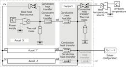
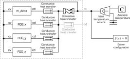
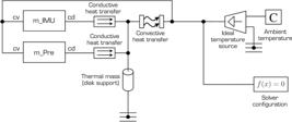
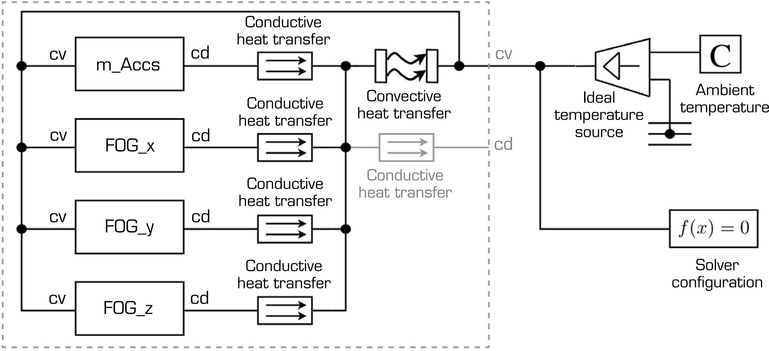
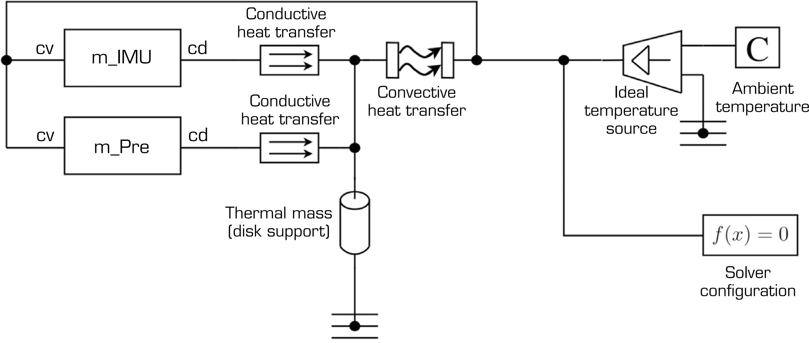
The remaining submodels are: (i) m_AccS (Fig. 22), composed of the components Acc_x, Acc_y, Acc_z, and support; (ii) m_IMU (Fig. 23), composed of the submodel m_AccS, components FOG_x, FOG_y, FOG_z, and support (thermal mass not explicitly shown but shared among FOGs); and (iii) the full model of SISNAV (m_Sd), with its submodels m_IMU and m_PrE, and disk support, shown in Fig. 24. As always, conductive heat transfer blocks are added cumulatively to each aggregated level.

Figure 22
Thermal simulation submodel m_AccS.

Figure 23
Thermal simulation submodel m_IMU.

Figure 24
SISNAV thermal simulation model m_SdU.

Full SISNAV model

Table 2 presents the HTC values of the SIMSCAPE “Convective heat transfer” block parameters, adjusted according to the hierarchical modelling level (component, submodel, and full model). After coupling the components, airflow and boundary conditions were modified, with internal surfaces losing exposure to ambient air and external regions showing reduced buoyancy. Consequently, most of the effective HTCs were adjusted to lower values, reflecting the reduced cooling efficiency of the stacked configuration and ensuring that simulated temperatures remained consistent with experimental results.

Table 2
Adjusted HTCs for each hierarchical level.

HTCs	Sd	m_PrE	m_IMU	m_AccS	Component
ProcSISNAV	3.5	6.0	-	-	6.0
EleGFO	2.1	2.1	-	-	2.2
Acc	6.0	-	6.0	6.0	6.0
AccS	6.0	-	6.0	-	-
IMU support	3.5	-	5.0	-	-
FOG_h	3.8	-	4.8	-	4.8
FOG_I	3.0	-	5.0	-	5.0

• Source: Elaborated by the authors.

Theoretical/effective HTC

In natural convection, the heat-transfer coefficient h is inherently temperature-dependent through the Rayleigh and Grashof numbers and therefore varies with the body ambient temperature difference ∆T. Classical correlations provide the theoretical local value for an idealized surface directly exposed to air.

However, within the context of lumped thermal modelling, such as the SIMSCAPE convective heat transfer block, the full geometric and material complexity of the assembly (resistors, PCB, enclosure walls, interfaces) collapses into a single thermal node representing the outer surface. Consequently, a constant effective convective coefficient is required to reproduce the steady-state temperature rise observed in the physical system. In this work, this effective coefficient is related to the global energy balance h_eff = Q A^-1 ΔT^-1, where Q is the dissipated power, A is the external area of the enclosure, and ∆T the measured (or simulated) steady-state temperature difference.

The parameter h_eff should not be interpreted as a theoretical convection coefficient; instead, it aggregates the internal thermal resistances between the heat source and the outer surface of the enclosure, together with non-uniform surface temperatures, enclosure geometry, and additional heat-transfer mechanisms (e.g., radiation or structural conduction).

Example: EleGFO

Given Q = 2.168 W, A = 0.082241 m² (measured by CAD software), and ∆T = T_s - T_amb, where T_s = (35.938 + 273.15) K = 309.088 K (Fig. 17) and T_amb = (24 + 273.15) K = 297.15 K, then h_eff = Q A^-1 ∆T^-1 = 2.208 W m^-2 K^-1 (compare with the adjusted EleGFO component HTC value in Table 2). For the theoretical computation, one considers Eq. 7, suited to vertical plates (Incropera 2006), with L = 0.02492 (m) (EleGFO box height), g = 9.81 (m s^-2) (gravitational acceleration), and (values picked around the {T_s , T_amb} range) k = 0.026 W m^-1 K^-1 (air thermal conductivity), Pr = 0.71 (-) (Prandtl number) and ν = 1.6 × 10⁻⁵ m² s^-1 (air kinematic viscosity). Computing h_theo gives the value of 6.798 W m^-2 K^-1.

(7) $\begin{array}{c}{h}_{theo}=k\frac{Nu}{L}withNu=0.68+\frac{0.670R{a}^{\frac{1}{4}}}{{[1+{\left(\frac{0.492}{Pr}\right)}^{\frac{9}{16}}]}^{\frac{4}{9}}},Ra=Gr\ast \mathrm{Pr},\\ Gr=\frac{g\beta (T_s-T_{amb})L^3}{v^2}and\beta =\frac{1}{\frac{1}{2}(T_s+T_{amb})}\end{array}$

Where Nu, Ra, Gr, and Pr are respectively Nusselt, Rayleigh, Grashof, and Prandtl numbers.

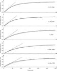
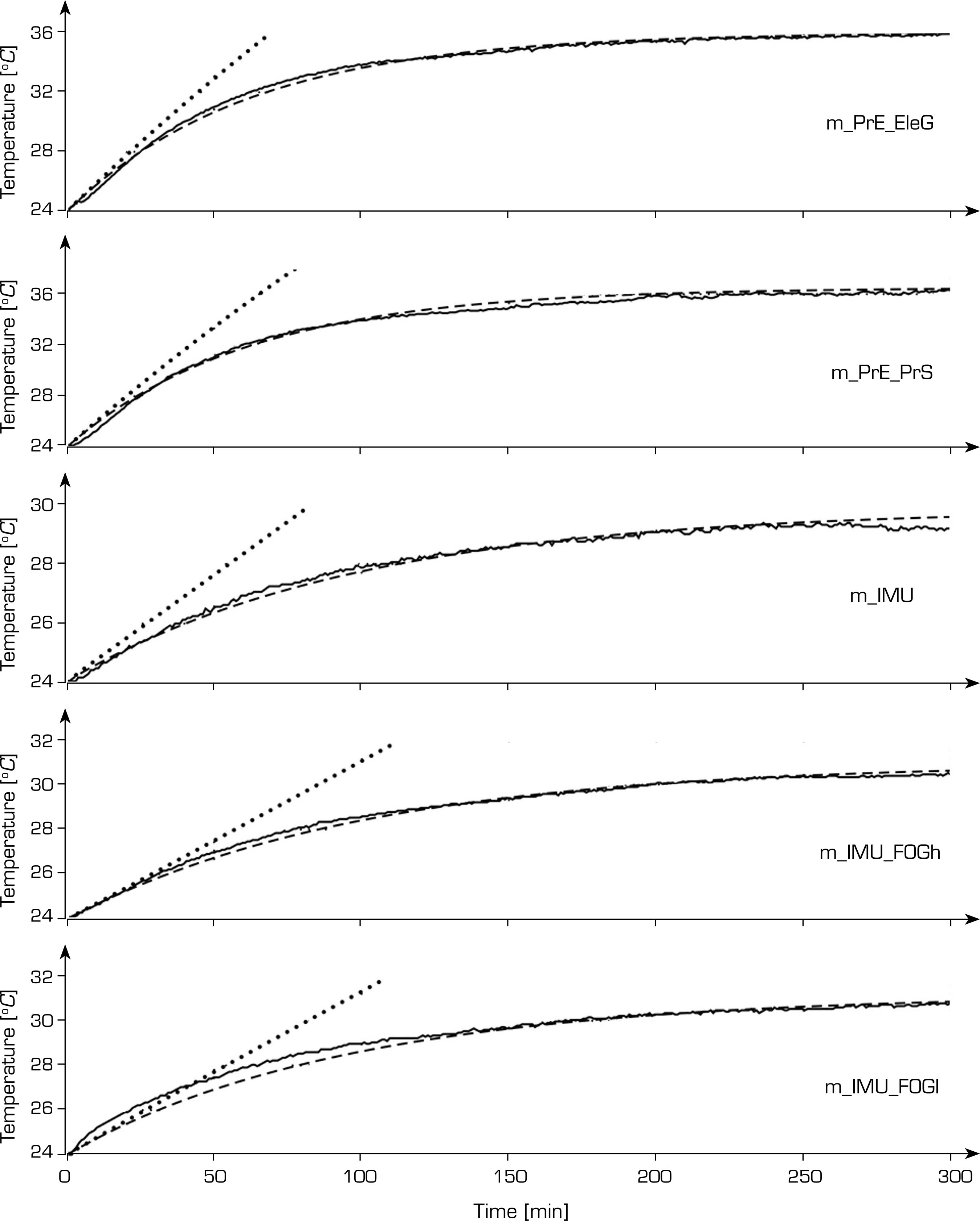
The results of the M&I procedure are presented in Figs. 17, 25, and 26, which correspond to non-aggregated components (e.g., EleGFO, ProcSISNAV, Acc, FOG_x and FOG_y), submodel components (e.g., m_PrE_EleG, where EleGFO is part of the submodel m_PrE), and fully aggregated components (e.g., m_Sd_PrS, where ProcSISNAV – alias PrS – is part of the full model m_Sd), respectively.

Figure 25
Thermal submodel results and real data comparison. Continuous line = measurement; dashed = simulated; dotted = simulated (HTCs ≈ 0 W m-2 K-1).

Figure 26
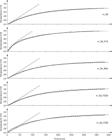
SISNAV thermal model results and real data comparison. Continuous line = measurement; dashed = simulated; dotted = simulated (HTCs ≈ 0 W m-2 K-1).

Figure 17 indicates that the highest temperatures are observed in the FOGs, followed closely by the power supply (EleGFO) and the SISNAV processor (ProcSISNAV); the power dissipation of the accelerometers is significantly lower. Figure 25 reveals the temperature equalization of the components within the submodel m_PrE, stabilizing around 36 °C, with ProcSISNAV exhibiting slightly higher temperatures. Conversely, the temperatures of both FOGs decrease substantially when integrated with the IMU support, which possesses a high metallic mass. Finally, Fig. 26 illustrates the effect of combining all submodels, where most components exhibit temperatures around 32 °C, while the ProcSISNAV (aggregated as m_Sd_PrS) shows a temperature approximately 2 ^oC higher than that value. The FOGs experience a slight temperature increase due to the thermal heating shared by the m_Sd_PrS across the entire submodel m_Sd.

Furthermore, the highest errors between simulated and experimental data came from the FOGs and, consequently, EleGFO (which delivers power to them). It was somehow expected, given the already mentioned unknown behavior of the FOGs’ temperature control circuitry. If one could feed the actual FOGs power profile into the “Power supply” block of their simulation models, then these errors could probably be minimized.

Comments on the procedure

Dividing the entire system into smaller parts and then joining them progressively was the key to obtaining a simple and intuitive process of M&I. This hierarchical approach tunes a few parameters at each step, not only during the full procedure, but also for local substitutions of system components and/or submodels.

The chosen simulation and experimental environments helped in the sense of providing data so that their matching feeds back into the parameter tuning process. The former relies on MATLAB, an established mathematical platform in the scientific community. Conversely, Arduino brings a recent framework aiming at easy-to-build experimental setups.

The model parametrization was mostly focused on tuning the conductive and convective heat transfer values required at the interface surfaces and the surrounding environment of the individual components, which facilitated the M&I procedure. Portions of certain convective areas were reallocated as conductive ones when forming each submodel.

Regarding the selected light-gray color box, the substitution or addition of individual system components is straightforward, generally resulting in a simple update of the affected thermal models and local adjustments. Furthermore, these models can be enhanced with additional blocks to ensure that their simulation outputs align more closely with the respective measurements. One example is the dependency of FOG power consumption on temperature, as mentioned earlier.

Other benefits obtained or perceived from the specific procedure described in this work were: (i) the agility and quickness to build and execute each of the defined steps; (ii) the flexibility and ease in adjusting parameters; (iii) the low demand and cost for human and material resources (MATLAB could be replaced by its free alternative OCTAVE, if necessary); and (iv) even more reduced work and cost for posterior replacement and retuning of system components or submodels.

CONCLUSION AND FUTURE WORK

This work proposed a methodology for M&I, outlining four steps to conceive, develop, verify, and validate a given system or set of components. The methodology is illustrated with a practical example, where physical modelling was implemented from a light-gray box perspective. Full SI was achieved progressively by aggregating each component or submodel and tuning the respective interfacing parameters. The results were presented alongside the respective measurements, demonstrating good agreement with the simulation data in each of the aggregation phases.

The complement of this work may comprise (i) an experiment with the full and updated SISNAV model (considering its current metallic case) to obtain internal temperature measurements and tune the full thermal model parameters, (ii) the presentation of results from environmental qualification tests and their comparison with the respective model simulation data, (iii) the presentation of the results of a rocket launch campaign under known weather conditions, (iv) the use of computational intelligence to automatically tune the parameters (e.g., Ramos (2011)), and (v) the application of inverse-modelling techniques to evaluate the obtained parameters.

ACKNOWLEDGEMENTS

To Instituto de Aeronáutica e Espaço, for all the support received from the Laboratory of Identification, Control and Simulation, given by its technical staff, which supplied equipment and the SISNAV itself.

• DECLARATION OF USE OF ARTIFICIAL INTELLIGENCE TOOLS
  In the preparation of this manuscript, the AI tool “ChatGPT” was utilized as an aid for search engines querying of academic work associated with literature review.
• FUNDING
  This research received no specific grant from any funding agency in the public, commercial, or not-for profit sectors.
• Peer Review History:
  Single Blind Peer Review.

DATA AVAILABILITY STATEMENT

Simulation parameters and experimental data can be obtained from the corresponding author upon request.

REFERENCES

• Chen C, Pan X (2023) Deep learning for inertial positioning: a survey. IEEE Trans Intell Transp Syst 25 (9). https://doi.org/10.1109/TITS.2024.3381161
  » https://doi.org/10.1109/TITS.2024.3381161
• El-Sheimy N, Youssef A (2020) Inertial sensors technologies for navigation applications: state of the art and future trends. Satell Navig 1(2):1-17. https://doi.org/10.1186/s43020-019-0001-5
  » https://doi.org/10.1186/s43020-019-0001-5
• Gonzáles-Bárcena D, Cavia-Fraile S, Torralbo I, Borque C, Arroyo JM, Urdampilleta I, Solyga M, Peyrou-Lauga R (2024) Hierarchical thermal modeling and analysis automatization of Comet Interceptor Probe B2 with ESATAN-TMS. Paper presented 2024 53rd International Conference on Environmental Systems. ICES; Louisville, USA. https://ttu-ir.tdl.org/items/5dc26ddf-fe65-4fe7-adbd-cd4af1fffd55
  » https://ttu-ir.tdl.org/items/5dc26ddf-fe65-4fe7-adbd-cd4af1fffd55
• Incropera FP (2006) Fundamentals of heat and mass transfer. 6th ed. Massachusetts: John Wiley and Sons Inc.
• Isermann R, Münchhof M (2010) Identification of dynamic systems: an introduction with applications. Berlin: Springer.
• Jacobs ED (1972) Accelerometer. U.S. Patent 3702073. Filed February 28, 1969; issued November 7, 1972. [accessed January the 29^th 2026]. https://patents.google.com/patent/US3702073A/en
  » https://patents.google.com/patent/US3702073A/en
• Lapusan C, Balan R, Hancu O, Plesa A (2016) Development of a multi-room building thermodynamic model using SIMSCAPE library. Energy Procedia 85:491-499. https://doi.org/10.1016/j.egypro.2015.12.258
  » https://doi.org/10.1016/j.egypro.2015.12.258
• Lienhard VJH, Lienhard IV JH (2024) A heat transfer textbook. Version 6.00. 6th ed. Cambridge: Phlogiston Press.
• Liu H, Cai J, Kim D (2022) A hierarchical gray-box dynamic modeling methodology for direct-expansion cooling systems. Technical report. University of Oklahoma; Lawrence Berkeley National Laboratory. [accessed Jan 29 2026]. https://escholarship.org/uc/item/8kt412bk
  » https://escholarship.org/uc/item/8kt412bk
• Ljung L (1996) Development of system identification. Paper presented 1996 13th World Congress of IFAC. IFAC; San Francisco, USA. https://www.sciencedirect.com/science/article/pii/S1474667017581380
  » https://www.sciencedirect.com/science/article/pii/S1474667017581380
• Ljung L (1999) System identification: theory for the user. 2nd ed. New Jersey: Prentice Hall PTR.
• Lv Z, Sun Z, Wang L, Liu Q, Zhang J (2025) Multi-level thermal modeling and management of battery energy storage systems. Batteries 11(6). https://doi.org/10.3390/batteries11060219
  » https://doi.org/10.3390/batteries11060219
• MathWorks (2024) Build model of battery module with thermal effects. [accessed Jan 29 2026]. https://www.mathworks.com/help/simscape-battery/ug/build-battery-module-thermal-effects.html
  » https://www.mathworks.com/help/simscape-battery/ug/build-battery-module-thermal-effects.html
• MATLAB (2011) MATLAB. Version 7.12.0 (R2011a). Natick, MA: The MathWorks Inc.
• McFadden C (2017) The origin of the word engineering. [accessed Oct 25 2025]. https://interestingengineering.com/culture/the-origin-of-the-word-engineering
  » https://interestingengineering.com/culture/the-origin-of-the-word-engineering
• Mijlad A, Mezouar A, Benyahia S, Kherraz N (2016) Simscape electro-thermal modelling of the pin diode for power circuits simulation. IET Power Electron 9(12):2391-2398. https://doi.org/10.1049/iet-pel.2015.0340
  » https://doi.org/10.1049/iet-pel.2015.0340
• Ramos FO (2011) Automation of H∞ controller design and its observer-based realization (doctoral thesis). Instituto Nacional de Pesquisas Espaciais; Institut Supérieur de l’Aéronautique et de l’Espace. https://bdtd.ibict.br/vufind/Record/INPE_4f67369aef6932e3293f29199f60abcd
  » https://bdtd.ibict.br/vufind/Record/INPE_4f67369aef6932e3293f29199f60abcd
• Ramos FO (2015) History and current status of SISNAV: a brief report. Paper presented VIII Brazilian Symposium of Inertial Engineering. Instituto Nacional de Pesquisas Espaciais; São José dos Campos, Brazil. https://www.researchgate.net/publication/281068299_History_and_current_status_of_SISNAV_a_brief_report
  » https://www.researchgate.net/publication/281068299_History_and_current_status_of_SISNAV_a_brief_report
• Tannous PJ, Alleyne AG (2020) Multilevel hierarchical estimation for thermal management systems of electrified vehicles. J Dyn Syst Meas Control 142(11). https://doi.org/10.1115/DSCC2020-3175
  » https://doi.org/10.1115/DSCC2020-3175
• The Arduino Team (2024) What is Arduino? [accessed Oct 25 2025]. https://www.arduino.cc/en/about?utm_source=chatgpt.com
  » https://www.arduino.cc/en/about?utm_source=chatgpt.com
• Wang Q, Li Y, Niu X (2016) Thermal calibration procedure and thermal characterisation of low-cost inertial measurement units. J Navig 69(2):373–-390. https://doi.org/10.1017/S0373463315000600
  » https://doi.org/10.1017/S0373463315000600

Edited by

• Section editor:
  Marcia Mantelli https://orcid.org/0000-0002-6276-8993

Publication Dates

• Publication in this collection
  13 Mar 2026
• Date of issue
  2026

History

• Received
  23 Apr 2025
• Accepted
  26 Jan 2026