Forecasting natural gas consumption in a cement plant – a case study

Previsão do consumo de gás natural em uma fábrica de cimento – estudo de caso

Abstract

Abstract  This study aims to investigate the forecasting of natural gas consumption in a cement plant in Rio de Janeiro, amidst the transition from the regulated to the open natural gas market, contextualized in the Brazil’s “new gas law” policies. We use demand forecasting to potentially reduce gas acquisition, transportation, and storage costs in the transport pipeline grid. For this purpose, the company’s historical daily demand data has been collected, as well as other exogenous data on related daily time series, all to be used in the training of univariate and multivariate forecasting models. The univariate models fitted in this study are the Naïve Method, Mean Method and Holt-Winters models. The multivariate forecasting models are dynamic regression and SARIMAX models, both of which link the target time series with the external-related ones. After training, these models are used to make predictions on the validation data period, and their accuracy is compared between themselves over five different accuracy metrics, thus highlighting the performance and suitability of each model. The results indicate that multivariate models present significantly better accuracy compared to univariate ones in the test period. The best results from the multivariate models present a MAPE value of 9.9% and an MPE of -0.3%.

Keywords:
Demand forecasting; Natural gas; Time series; Open gas market

Resumo

Resumo  Este estudo tem como objetivo investigar a previsão do consumo de gás natural em uma fábrica de cimento no Rio de Janeiro, no contexto da transição do mercado regulado para o mercado livre de gás natural, conforme as diretrizes da “nova lei do gás” no Brasil. Utiliza-se a previsão da demanda como ferramenta potencial para reduzir os custos de aquisição, transporte e armazenamento de gás na malha de gasodutos. Para isso, foram coletados dados históricos diários de consumo da empresa, bem como outras séries temporais diárias relacionadas, a serem utilizadas no treinamento de modelos de previsão univariados e multivariados. Os modelos univariados ajustados neste estudo são o Método Ingênuo (Naïve), o Método da Média e o modelo de Holt-Winters. Os modelos multivariados de previsão são um modelo de regressão dinâmica e modelos SARIMAX, ambos conectando a série temporal alvo com variáveis externas relacionadas. Após o treinamento, os modelos são utilizados para realizar previsões no período de validação, e sua acurácia é comparada entre sí por meio de cinco métricas diferentes, evidenciando o desempenho e a adequação de cada modelo. Os resultados indicam que os modelos multivariados apresentam uma acurácia significativamente superior em comparação aos univariados no período de teste. Os melhores resultados entre os modelos multivariados apresentam um valor de MAPE de 9.9% e de MPE de -0.3%.

Palavras-chave:
Previsão de consumo; Gás natural; Séries temporais; Mercado livre de gás

1 Introduction

The enactment of the New Gas Law (Law No. 14.134 of April 8, 2021) represents a significant milestone for the Brazilian natural gas market. This law, designed to promote competitiveness, reduce costs, and attract new investments, holds the potential to transform the industry. It follows the "New Gas Market" program launched by the Federal Government in 2019, which aims to establish a more dynamic and integrated market aligned with international best practices (Brasil, 2021).

The new legislation aims to unbundle the market, allowing the entry of new players and facilitating access to essential infrastructure, such as pipelines. This change is crucial to improving the competitiveness of the sector and aligning with global trends in more open and diversified markets (Empresa de Pesquisa Energética, 2021).

These transformations are expected to increase the supply and reduce the costs of natural gas in Brazil. They also promise to foster investments in infrastructure and enhance the competitiveness of the national industry in various sectors such as petrochemicals, metallurgy, and thermoelectric generation (Brasil, 2021).

In this new market context, the predictability of gas demand is more crucial than ever for consumers. Before this market shift, natural gas consumers would not have had the option to be involved in natural gas logistics or upstream supply, only being relegated to a passive consumer role. As such, forecasting internal natural gas demand would not be as relevant a necessity due to this limited autonomy. In the new paradigm, accurate demand forecasting is not just a planning tool, but a strategic necessity. It ensures that enough gas is available to meet consumer needs without supply interruptions, and helps optimize the operation of distribution networks, minimizing operational costs and avoiding resource waste (Liu et al., 2023).

For this reason, it is of strategic interest to make demand forecasts based on consumer historical curves. Time series forecasting models can be used to do this, and they are trained on existing demand data and related time series.

This analysis will cover a case study of a cement factory in Rio de Janeiro consuming natural gas. The aim is to train forecasting models on a daily demand time series using historical data and other exogenous time series. The univariate models will be the Naïve Method, the Mean Method and the Holt-Winters. As for the multivariate models, one will be fitted through a dynamic regression approach, and the other will be based on a seasonal auto-regressive integrated moving-average model utilizing exogenous variables (SARIMAX). These models will be tested over the same validation period, and their results will be compared.

To make and evaluate these forecasts, firstly, this study will present an exploratory analysis of the historical daily demand data, including an autocorrelation analysis, looking for trends and seasonality in the series. Afterwards, the previously mentioned univariate forecasting models will be adjusted and fitted using the insights obtained from the exploratory analysis. A similar process is then conducted for the multivariate models, with a cross-correlation analysis being performed between the new added exogenous daily time series and the historical demand series that will support the fitting of the dynamic regression and SARIMAX models. Five different accuracy metrics are then listed on their pros and cons and proposed to evaluate the performance of the forecasting models. All forecasting models will then be tested over a validation interval of the data corresponding to the latter 20% of the historical demand series, the forecasts are all made on a rolling manner on a D+1 basis, where each prediction is made in a daily basis and only for the next day. Finally, after constructing the testing predictions, their performance is compared to each other and some final conclusions are drawn.

2 Literature review

Natural gas demand forecasting has been extensively studied due to its critical role in energy planning, supply chain management, and economic decision-making. The literature has explored various forecasting methodologies, ranging from traditional statistical techniques to advanced machine learning models. This section presents an overview of key contributions in the field.

Early natural gas demand forecasting works predominantly relied on classical statistical models such as Autoregressive Integrated Moving Average (ARIMA) and its variations. For instance, Box & Pierce (1970) introduced the ARIMA framework, which has since become a cornerstone in time series forecasting. Studies such as Pindyck (1999) effectively applied ARIMA models to capture seasonality and economic trends in natural gas pricing and consumption.

Machine learning methods have gained prominence with the increasing data availability and computational power. Hastie et al. (2009) provided a comprehensive foundation on machine learning techniques, including regression trees, random forests, and support vector machines (SVM), which have been successfully applied in gas demand forecasting. For example, Hong (2009) demonstrated the superior performance of support vector regression (SVR) in predicting electric load demand compared to traditional methods.

More recent advancements incorporate deep learning architectures such as recurrent neural networks (RNNs) and long short-term memory (LSTM) networks into forecasting energy demands. Zhou et al. (2022) applied LSTM models to improve forecast accuracy for natural gas and electricity consumption in China, showing improved performance in capturing temporal dependencies.

Combining traditional statistical methods with machine learning models has emerged as a promising strategy. Zhang (2003) proposed a hybrid ARIMA-ANN model that leverages the strengths of both approaches. Such hybrid models have improved accuracy by simultaneously capturing linear and non-linear patterns. This study laid much of the groundwork for subsequent research on forecasting techniques utilizing Neural Networks and deep learning methods.

Soldo et al. (2014) has explored auto-regressive forecasting models to forecast day-ahead residential natural gas consumption, utilizing exogenous variables such as solar radiation. This approach is similar to the one proposed in this study in many ways.

In light of these studies, this paper focuses on applying classical forecasting methodologies in a more didactic way in an industrial setting on a day-ahead basis and utilizing exogenous explanatory variables. In this manner, it also aims to establish more scientific approaches to decision-making and forecasting in the developing new open gas market in Brazil, where agents are only beginning to take accountability for the management of natural gas supply and transportation and where the literature has not yet developed to real base cases.

3 Materials and methods

To carry out this study, a series of critical information and definitions must be outlined in stages according to the following descriptions.

3.1 Target time series analysis

Relevant data must be collected and processed for training and validating the time series forecasting models. The company provided a dataset with 972 observations containing historical daily time series from February 1, 2021, to September 30, 2023.

This dataset includes a time series of interest for this study, the Realized Daily Quantity (RDQ), which highlights the volume in cubic meters of natural gas consumed daily. This series will be forecasted in this study.

This series is divided between training and validation periods, representing 80% and 20% of the dataset's observations. The training period will be used to fit and adjust the forecasting models, while the validation period will be used to simulate forecasts from the trained models and comparatively measure their performance.

The company's RDQ (Figure 1) is analyzed. To train the forecasting models as accurately as possible, trends, seasonality, and abnormal behaviors in the target series must be detected.

Figure 1
Historical natural gas demand curve (RDQ) [m³/day].

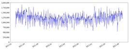
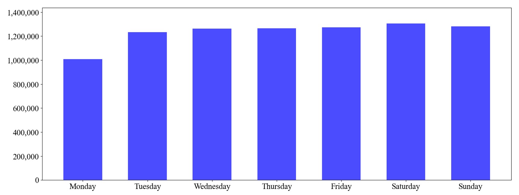
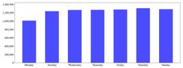
From the raw data, the average demand during the period is 1,233,061 m³/day, with a minimum of 534,887 m³/day and a maximum of 1,904,930 m³/day. However, demand on Mondays is much lower than on all other weekdays (Figure 2). This fact is consistent with the information available that the company's factory performs preventive maintenance on Mondays, temporarily and partially halting the kilns during these processes. The series also shows a standard deviation of 219,336 m³/day.

Figure 2
Average RDQ by weekday [m³/day].

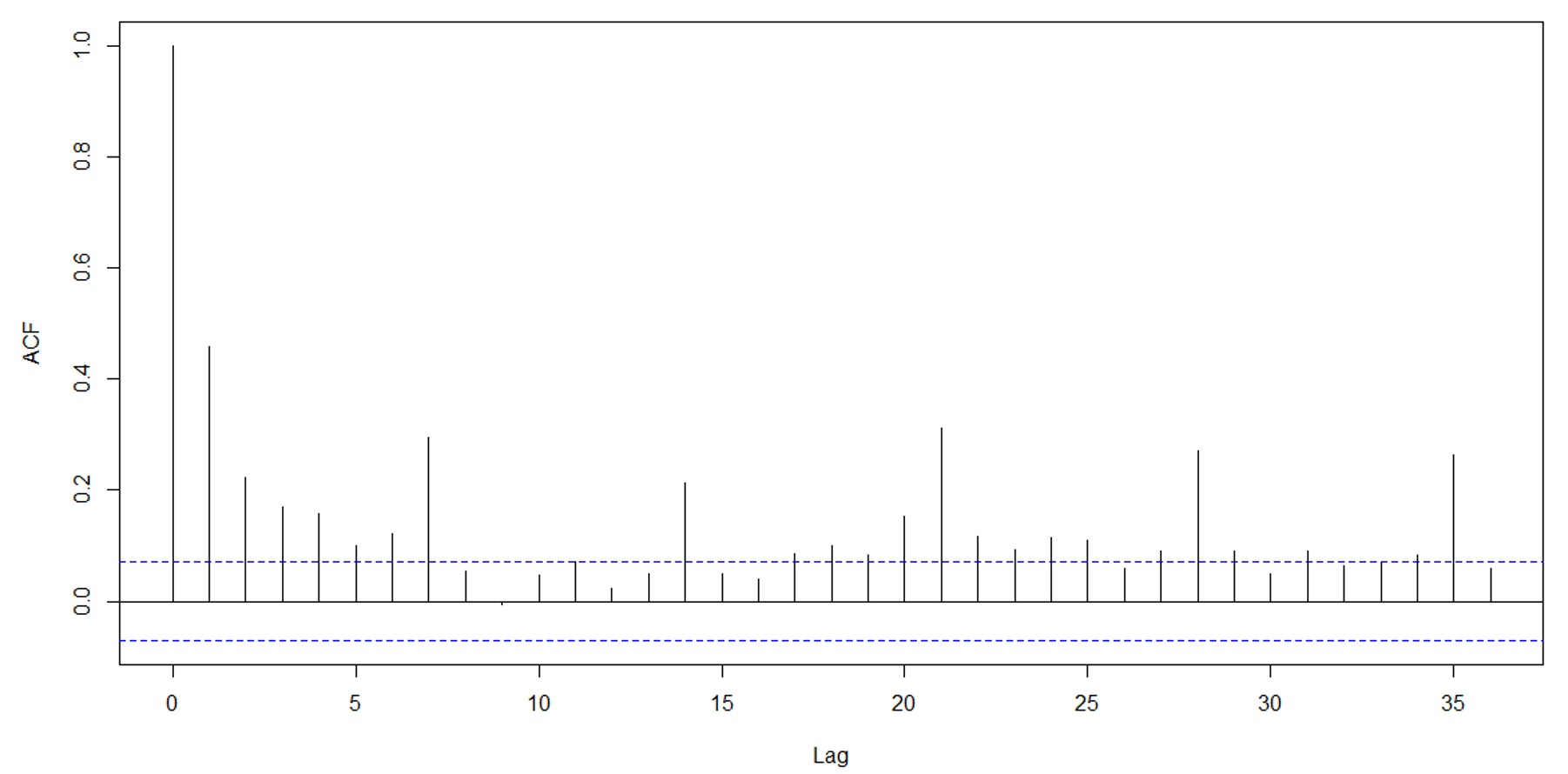
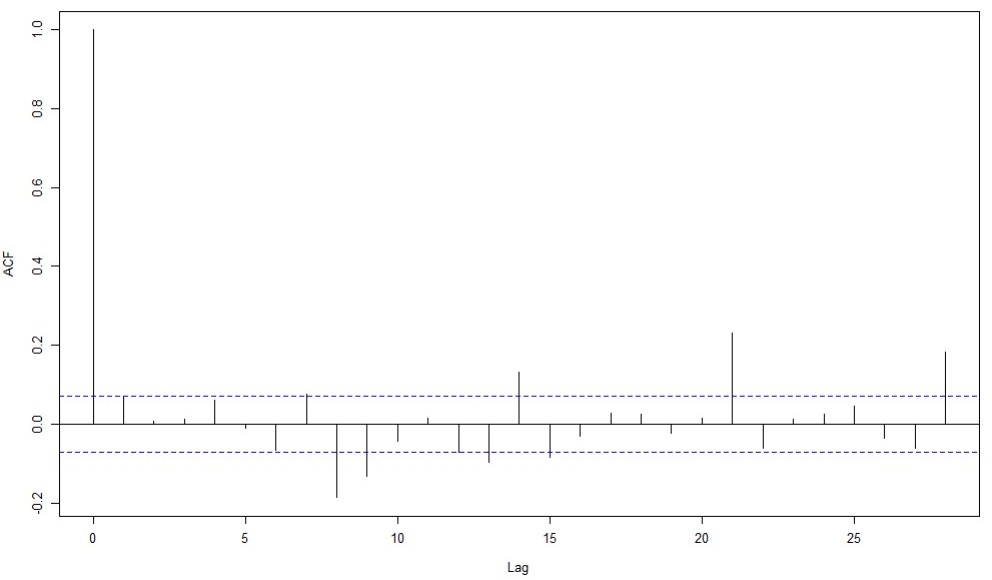
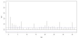
Additionally, an autocorrelation function (ACF) (Venables & Ripley, 2002) is performed to identify patterns of seasonality and trend in the series thoroughly. The ACF measures correlation values between the target series and its lags (previous time steps).

The ACF result presents values above the significance threshold for values below lag 5 and multiples of lag 7 (Figure 3). These values in the ACF may indicate a slight growth trend and the presence of weekly seasonality, likely caused by the previously mentioned preventive maintenance events on Mondays.

Figure 3
Autocorrelation function of the target series.

3.2 Univariate models

The univariate forecasting models are fitted and adjusted around the base time series analysis and ACF results. At this point in the study, three forecasting models are selected.

Firstly, the Naïve method, the forecast model follows the same value as the last observation in the time series, adhering to the following formulation (Hyndman & Athanasopoulos, 2018):

${\widehat{Z}}_{T+h}=Z_T$ (1)

where:

${\widehat{Z}}_{T+h}=forecast\mathrm{}for\mathrm{}{Z}_t\mathrm{}made\mathrm{}at\mathrm{}time\mathrm{}T\mathrm{}for\mathrm{}horizon\mathrm{}h$

$Z_T=the\mathrm{}last\mathrm{}observation\mathrm{}of\mathrm{}a\mathrm{}time\mathrm{}series$

In this case, the only relevant parameter for model adjustment is the definition of $Z_T$, which is equal to 1,006,760 NG m³/day for the last observation in the training period. Consequently, the Naive model's forecasts for the validation period will start with this value for the first D+1 prediction and later will always replicate the last day’s RDQ value for the next D+1 forecast cycle in accordance with Equation 1.

The Mean Method forecast model is also selected; here, the forecast will follow the average value of all observations of the target time series up to the forecasted observation (Hyndman & Athanasopoulos, 2018). Thus, it follows the following equation:

${\widehat{Z}}_{T+h}=\frac{1}{T}\sum _{t=1}^T{Z}_t$ (2)

In this method, the forecast for the first day of the validation period will equal the average of the observations in the training period, which in this case is 1,215,337 NG m³/day. As new D+1 forecasting cycles in the validation period are added and new previous days' RDQ values are observed, the average of the historical values that compose the D+1 forecast will be recalculated accordingly.

Holt-Winters is the last univariate forecasting method used. This method applies exponentially decreasing weights to past observations, producing forecasts that capture short-term trends and patterns by calculating a weighted average of past values, where weights decrease as data age.

There are three main variations of the exponential smoothing method: Simple Exponential Smoothing (SES), Holt’s Model (Holt, 2004), and the Holt-Winters Model (Winters, 1960). In this case study, the ACF analysis (Figure 3) of the target time series indicated the presence of seasonality but not a trend, so the Holt-Winters model is chosen, as it is more suitable for time series with these seasonal characteristics (Winters, 1960). The equations for this model are as follows:

${\widehat{Z}}_{T+h}=N_t+h{T}_t+S_{t+h-m\left(k+1\right)}$ (3)

where:

$N_t=\alpha \left(Z_t-S_{t-m}\right)+(1-\alpha )(N_{t-1}+T_{t-1})$ (4)

$T_t=\beta \left(N_t-N_{t-1}\right)+\left(1-\beta \right)T_{t-1}$ (5)

$S_t=\gamma \left(Z_t-N_{t-1}-T_{t-1}\right)+\left(1-\gamma \right)S_{t-m}$ (6)

$N_t=level\mathrm{}of\mathrm{}the\mathrm{}series\mathrm{}at\mathrm{}time\mathrm{}t$

$T_t=trend\mathrm{}of\mathrm{}the\mathrm{}series\mathrm{}at\mathrm{}time\mathrm{}t$

$S_t=seasonality\mathrm{}of\mathrm{}the\mathrm{}series\mathrm{}at\mathrm{}time\mathrm{}t$

$\alpha =smoothing\mathrm{}parameter\mathrm{}for\mathrm{}the\mathrm{}level\mathrm{}(0\le \alpha \le 1)$

$\beta =smoothing\mathrm{}parameter\mathrm{}for\mathrm{}the\mathrm{}trend\mathrm{}(0\le \beta \le 1)$

$\gamma =smoothing\mathrm{}parameter\mathrm{}for\mathrm{}the\mathrm{}seasonality\mathrm{}(0\le \gamma \le 1)$

$k=mod\left(\frac{h-1}{m}\right)$ (7)

$h=forecast\mathrm{}horizon$

$m=length\mathrm{}of\mathrm{}seasonal\mathrm{}cycle$

The model fitting process obtains the model’s parameters α, β e γ by minimizing the sum of squared errors between the calibrated model and the target series values during the training period. In this case, the regression results indicate $\alpha =0.19$, $\beta =0.0$ and $\gamma =1.0$, to be implemented in Equations 4-6. The regression process also detects no trend but perceives apparent seasonality with $m=7$.

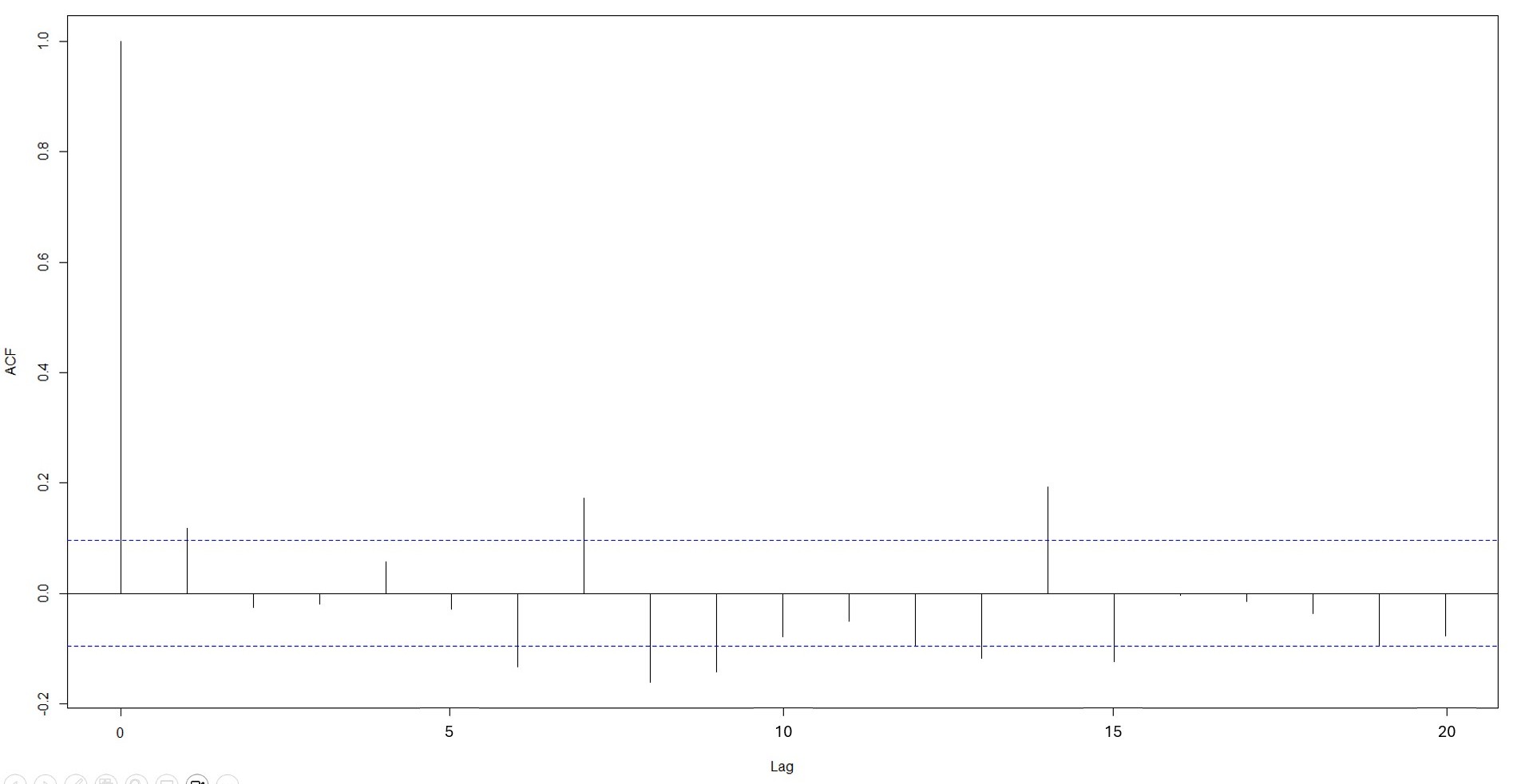
Testing the Holt-Winters fitted model for residuals autocorrelation in the training period (Figure 4) demonstrates that there are still significant values in the lag = 7 multiples, indicating that the fitted model does not fully capture the series' weekly seasonal behaviour.

Figure 4
Autocorrelation function of Holt-Winters model residuals.

Running an Autoregressive Conditional Heteroskedasticity (ARCH) (Engle, 1982) test in the model’s residuals returns a p-value of 3.8e-5, rejecting the null hypothesis and demonstrating that the variance of residuals changes over time.

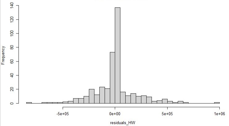
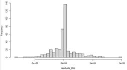
In sequence, the residuals are tested for normality, beyond analyzing the histogram of residuals visually for compatibility (Figure 5), a Jarque-Bera (Jarque & Bera, 1980) test is run over the residuals, resulting in a p-value of 2.2e-16, indicating that the residuals do not fit into a normal distribution.

Figure 5
Histogram distribution of Holt-Winters model residuals.

3.3 Multivariate models

Beyond the univariate models, multivariate forecasting models for the target time series are developed using three additional daily time series as explanatory variables. The forecasting models to be trained are a Dynamic Regression and SARIMAX framework models. The exogenous series are as follows:

• Exchange Rate R$ - US$ (daily closing) FX [R$/US$]

• Brent Crude (daily futures) BRENT [US$/bbl]

• Dow Jones U.S. Non-Ferrous Metals Index DJUSNF [-]

These additional time series (Investing.com, 2024a, 2024b, 2024c) were chosen based on the authors’ technical and commercial knowledge and experience. As such, these choices rely on somewhat subjective perspectives. In the preprocessing analysis, no outliers needed to be removed from any time series, as all values are real and don’t distort the overall analysis results.

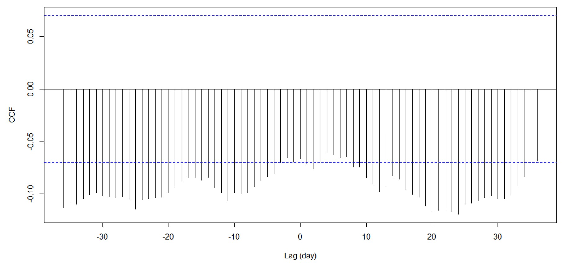
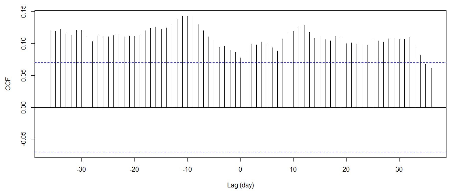
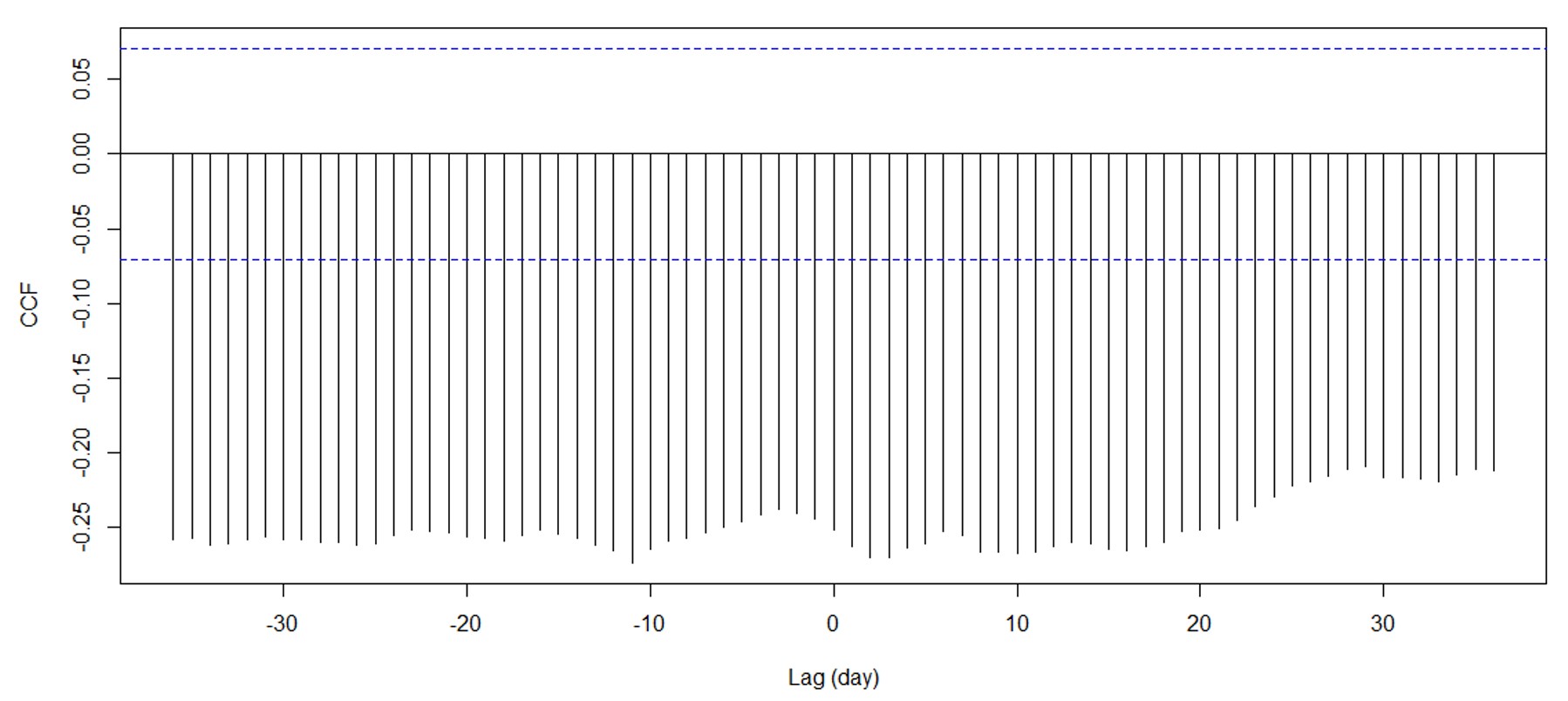
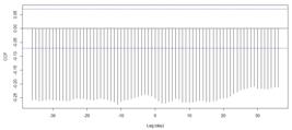
To identify functional relationships between the explanatory and the target series and construct the multivariate forecasting models, the cross-correlation function (CCF) (Venables & Ripley, 2002) must be calculated between all exogenous variables and the target series. The CCF follows the same formulation as the autocorrelation function (ACF), but instead of calculating correlations between lags of the same series, it calculates correlations between lags of different time series. Three CCF analyses are performed, one for each explanatory series in the dataset.

Among these results, only the correlation values for negative lags between series will be relevant for the regression, as the forecast cannot benefit from future values of other series at the time of the D+1 forecast.

Overall, the CCFs show relatively low values, ranging from -0.30 to 0.15 (Figures 6-8), but they do present values beyond the significance threshold across all combinations.

Figure 6
Cross-Correlation Function (RDQ – DJUSNF).

Figure 8
Cross Correlation Function (RDQ – FX).

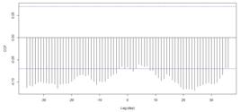
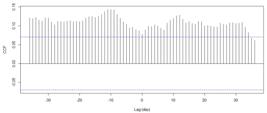
For the multivariate model, it is shown that the most significant relationship between the lagged variables is in the RDQ – Brent relation.

For the dynamic regression model (Lütkepohl et al., 1999), the fitting process will be based on the results of the CCFs (Figures 6, 7, 8) and the ACF results for the target series (Figure 3). The fitted model must be structured by considering the lags that showed significant correlations between time series. The dynamic regression allows for including the exogenous variables’ past values (only negative lags) to capture these significant correlations. The model follows the formulation:

${RDQ}_t={\alpha }_0+{\sum }_l^{}{\eta }_l{RDQ}_{t-l}+{\sum }_k^{}{\alpha }_k{DJUSNF}_{t-k}+{\sum }_j^{}{\beta }_j{BRENT}_{t-j}+{\sum }_m^{}{\gamma }_m{FX}_{t-m}+{ϵ}_t$ (8)

where:

${RDQ}_t=Realized\mathrm{}Daily\mathrm{}Quantity\mathrm{}\left(target\mathrm{}series\right)$

${DJUSNF}_t=Dow\mathrm{}Jones\mathrm{}U.S.\mathrm{}Non-Ferrous\mathrm{}Index$

${BRENT}_t=Brent\mathrm{}Crude\mathrm{}Daily\mathrm{}Futures$

${FX}_t=USD-BRL\mathrm{}exchange\mathrm{}rate\mathrm{}(closing,\mathrm{}selling)$

${\alpha }_0=Intercept$

${\eta }_l=lag\mathrm{}coefficients\mathrm{}of\mathrm{}{RDQ}_t$

$l\to index\mathrm{}of\mathrm{}target\mathrm{}series\mathrm{}lags\mathrm{}with\mathrm{}significant\mathrm{}correlation\mathrm{}values$

${\alpha }_k=lag\mathrm{}coefficients\mathrm{}of\mathrm{}{DJUSNF}_t$

$k\to index\mathrm{}of\mathrm{}significant\mathrm{}cross\mathrm{}lags\mathrm{}between\mathrm{}the\mathrm{}target\mathrm{}seiries\mathrm{}and\mathrm{}DJUSNF$

${\beta }_j=lag\mathrm{}coefficients\mathrm{}of\mathrm{}{BRENT}_t$

$j\to index\mathrm{}ofsignificant\mathrm{}cross\mathrm{}lags\mathrm{}between\mathrm{}the\mathrm{}target\mathrm{}seiries\mathrm{}and\mathrm{}BRENT$

${\gamma }_m=lag\mathrm{}coefficients\mathrm{}of\mathrm{}{FX}_t$

$m\to index\mathrm{}ofsignificant\mathrm{}cross\mathrm{}lags\mathrm{}between\mathrm{}the\mathrm{}target\mathrm{}seiries\mathrm{}and\mathrm{}FX$

${ϵ}_t=error\mathrm{}term\mathrm{}~N(0\mathrm{},\mathrm{}{\sigma }^2)$

Figure 7
Cross-Correlation Function (RDQ – Brent).

Regarding the dynamic regression process itself, the initial regression to fit the model considers only the three most significant lag correlations for the target series ACF (Figure 3) and each CCF between variables as relevant intervals for the coefficients in the fitted model.

From this initial regression, the coefficients of the selected variable lags are adjusted to minimize the error in the training interval.

Once the coefficients are obtained, their significance levels are evaluated in the context of dynamic regression. If the p-value of at least one of the model coefficients is greater than 5% (which would indicate that the null hypothesis $H_0$: coef. = 0 cannot be rejected), the model is rejected, the variable with the least significant coefficient is removed, and the error minimization process is redone. This process is repeated until all the coefficients left in the model are significant.

After finishing the dynamic regression process, the results for the coefficients utilized in the multivariate model fitting are obtained and applied in Equation 8.

It is clear (Table 1) that the only significant relationship between different time series and the target series is given in the lagged BRENT correlation, which produces a coefficient in the multivariate model. This indicates a pattern over the training period where, when the price of natural gas increases (that being defined by the BRENT oil price), there would be a subsequent decrease in natural gas consumption.

Table 1
Parameters of the multivariate dynamic regression forecasting model.

Coefficient	Estimate	Std. Error	t-value	Pr (> | t |)
Intercept	5.630e+05	7.688e+04	7.323	6.15e-13
Lag (RDQ, -1)	4.121e-0.1	3.184e-02	12.946	< 2e-16
Lag (RDQ, -7)	2.213e-01	3.187e-02	6.944	8.15e-12
Lag (BRENT, -10)	-1.373e+03	4.535e+02	-3.028	0.00254

In this scenario, the model still presented an R² of 0.285, indicating that 28.5% of the changes in the target series are explained by variations in the selected lagged series, a value that is not significant.

Through the fitting process in the Dynamic Regression, the model’s residuals for the training period still show significant correlation values for multiples of lag=7 (Figure 9), similar to the analysis of the residuals done in the Holt-Winters model.

Figure 9
Autocorrelation function of the Dynamic Regression model residuals.

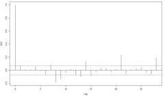
Checking the Dynamic Regression model’s residuals for Homoskedasticity through the Breusch-Pagan (Breusch & Pagan, 1979) test, provides a p-value of 7.9e-5, rejecting the null hypothesis of Homoskedasticity and indicating inconsistencies in the model’s fit.

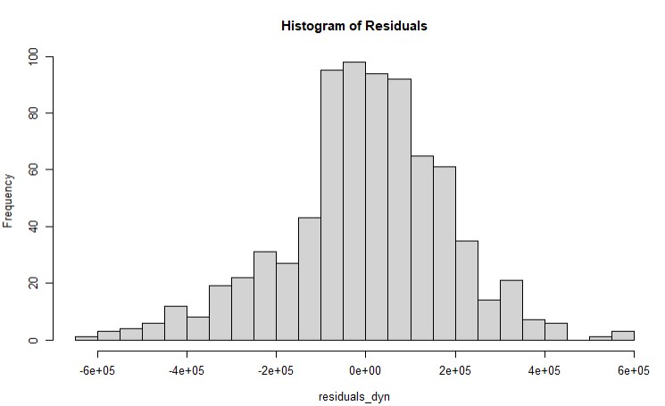
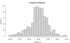
The residuals of the Dynamic regression model fit are tested for normality visually (Figure 10) and using the Jarque-Bera test. A p-value of 5.7e-7 in the test indicates that, although these residuals are closer to normality than the ones in the Holt-Winters model, they still cannot be considered a normal distribution, leaving room for better fits in other forecasting models.

Figure 10
Histogram distribution of the Dynamic Regression model residuals.

As the final forecasting model considered in this study, the SARIMAX model has been chosen. This is a variation of the autoregressive integrated moving average (ARIMA) model that considers seasonality (S) and exogenous variables (X). The model is molded by the $SARIMAX\left(p,d,q\right)\left(P,D,Q,s\right)$ parameters.

In the fitting process for the SARIMAX model over the training data, multiple sets of different configurations of the $\left(p,d,q\right)\left(P,D,Q,s\right)$ parameters are tested, with the coefficient regression realized over each configuration. At each configuration, the Akaike Information Criterion (AIC) is calculated. It gives a metric balancing the model’s fit with its own complexity to avoid overfitting. This becomes the primary metric for determining the model parameters. The configuration resulting in the lowest AIC value is the one utilized.

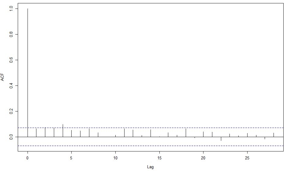
After the fitting process, the $SARIMAX\left(3,1,5\right)\left(2,0,2,7\right)$ configuration is selected, with an AIC value of 21,123.1. Analyzing the autocorrelation function for the SARIMAX model’s residuals (Figure 11), it becomes clear that this model is better fitted to capture the seasonality patterns than the previous regression-based models. This is likely due to the order 1 differentiation defined in the optimal model parameters.

Figure 11
Autocorrelation function of the SARIMAX model residuals.

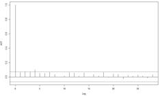
A Breusch-Pagan test is also conducted on the residuals to check their Homoskedasticity. This test results in a p-value of 0.00, rejecting the null hypothesis of Homoskedasticity and indicating that the model fit still has inconsistencies in the error distribution along the training interval.

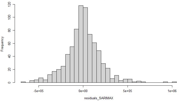
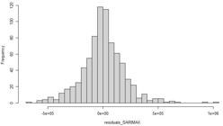
Checking for normality in the SARIMAX model presents the best fit visually (Figure 12) but still returns a 2.2e-16 p-value in the Jarque-Bera test, rejecting the hypothesis of normality.

Figure 12
Histogram distribution of the SARIMAX model residuals.

3.4 Accuracy metrics

To measure the performance of the models’ forecasts during the validation period, different error metrics will be used (Hyndman & Athanasopoulos, 2018). These include:

• ME – Mean Error

It is the average of the differences between the predicted and actual values. While it provides insight into systematic bias in the model, its primary limitation is that positive and negative errors can offset each other, potentially masking significant forecasting inaccuracies.

$ME=\frac{1}{n}\sum _{i=1}^n(y_i-\widehat{y_i})$ (9)

• RMSE – Root Mean Squared Error

Calculated from the square root of the average squared differences between predicted and actual values. It gives greater weight to more significant errors, making it highly sensitive to outliers. This characteristic makes RMSE particularly suitable when significant deviations from the mean are critical to detect.

$RMSE=\sqrt{\frac{1}{n}\sum _{i=1}^n(y_i-\widehat{y_i})²}\mathrm{}$ (10)

• MAE – Mean Absolute Error

It represents the average of the absolute differences between predicted and actual values. Unlike RMSE, MAE treats all deviations equally, providing a balanced measure of forecast accuracy. However, compared to RMSE, it may underestimate the impact of large errors.

$MAE=\frac{1}{n}\sum _{i=1}^n\left|y_i-\widehat{y_i}\right|$ (11)

• MPE – Mean Percentage Error

This metric calculates the average percentage errors, indicating the model's tendency to overestimate or underestimate values. Its primary drawback is sensitivity to extreme values, particularly when observed data points are near zero, which can distort the metric.

$MPE=\frac{1}{n}\sum _{i=1}^n\frac{y_i-\widehat{y_i}}{y_i}$ (12)

• MAPE – Mean Absolute Percentage Error

It computes the average absolute percentage difference between predicted and actual values. This metric is intuitive and facilitates straightforward interpretation across different scales. However, like MPE, it becomes unreliable when dealing with values near zero, as it can produce disproportionately large errors.

$MAPE=\frac{1}{n}\sum _{i=1}^n\frac{\left|y_i-\widehat{y_i}\right|}{y_i}$ (13)

Although other error metrics are included to add context to the results of this study, the MAPE will be the leading benchmark, as with series with all positive and significant values, it is still preferred as a factor of simplicity (Hyndman & Koehler, 2006).

3. Results

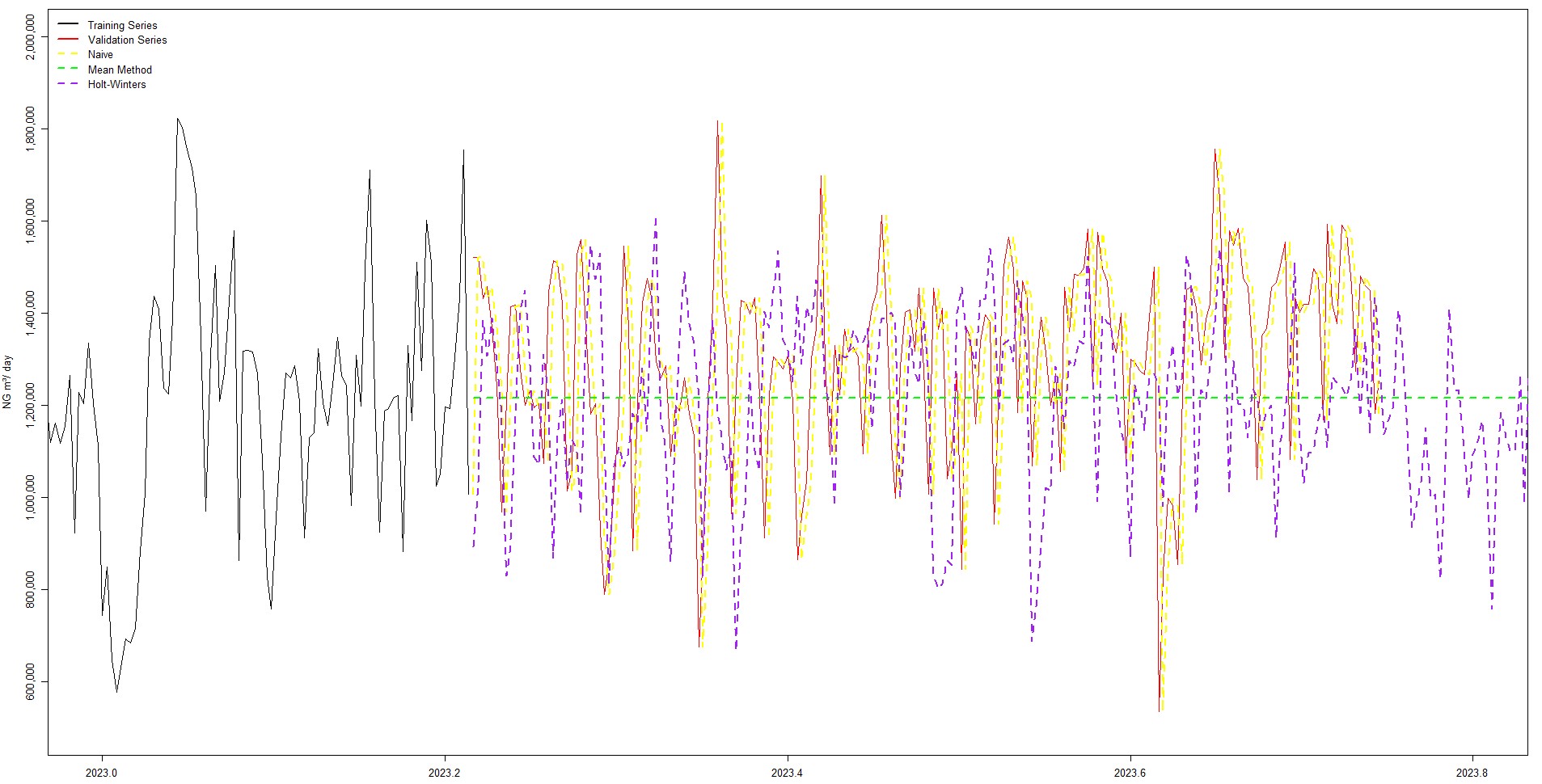
Initially, the univariate models—the Naive Model, the Mean Method Model, and the Holt-Winters Model—are forecasted through the validation period.

Visually (Figure 13.) the Holt-Winters fitted model performs best and follows the demand curve time series more closely.

Figure 13
Univariate model rolling starts forecasts inside the validation period.

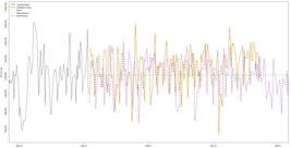
The multivariate model forecasts for the validation period are added at this point.

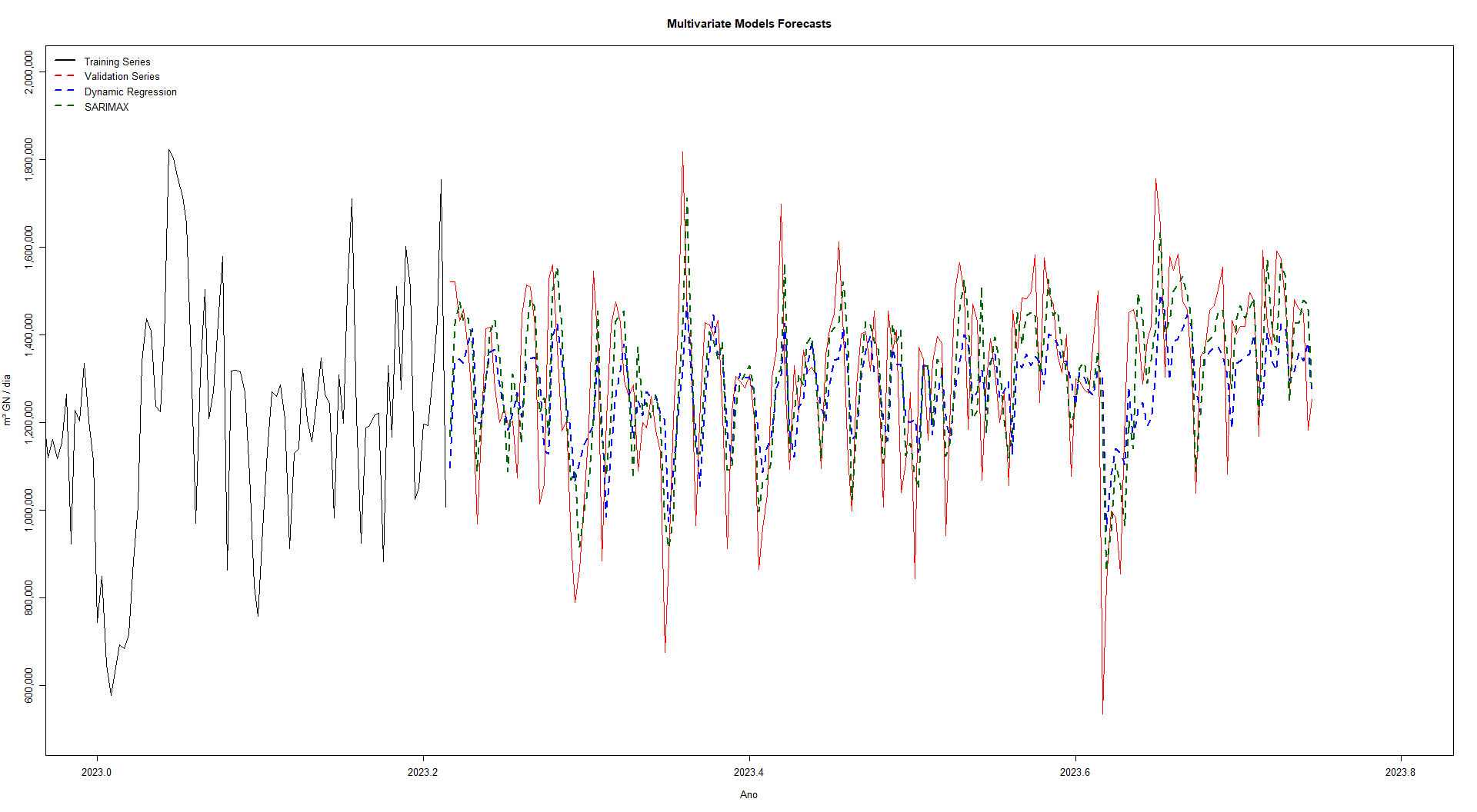
The perceived performance of the multivariate models (Figure 14), as it was with the Holt-Winters univariate model, follows the actual demand curve even closer.

Figure 14
Multivariate models rolling start forecast for the validation period.

For an analytical and objective comparative evaluation of each model’s performance, their predictions for the validation period are measured through the accuracy metrics previously described in the Materials and Methods section (Table 2).

Table 2
Accuracy metrics for all forecasting models in the validation period.

Model	ME	RMSE	MAE	MPE	MAPE
Naïve	1,267.5	219,027.8	163,073.8	-1.8%	13.9%
Mean Method	88,802.5	223,735.1	186,566.9	3.9%	14.9%
Holt-Winters	82,843.5	286,225.0	228,841.6	3.5%	18.4%
Dynamic Regression	27,068.8	181,299.1	141,811.4	-0.3%	11.8%
SARIMAX	562.8	158,905.6	119,930.9	-1.6%	9.9%

As the visual analysis revealed, the Multivariate Models present the best MAPE accuracy metrics among all proposed models in this study. Within the univariate models, there is one clear superior model, the Naïve model, presenting better accuracy and performance in all metrics.

4 Discussion

This study’s results suggest that a multivariate dynamic regression approach offers a solid improvement over univariate methods for forecasting daily natural gas demand in an industrial context. Still, the model shows difficulties in capturing the seasonality patterns that are better perceived in the SARIMAX model, which is corroborated by the model’s residuals correlation analysis and overall better accuracy scores in all metrics but the MPE. Multivariate models, especially those that incorporate external economic and market factors, capture complex interactions between time series variables more effectively, which aligns with findings from recent studies in natural gas forecasting. For example, machine learning models such as Long Short-Term Memory (LSTM) networks, which handle sequential dependencies, have shown enhanced predictive power in other markets with dynamic patterns. Integrating economic indicators like Brent crude prices can further improve forecasting accuracy, as these indicators frequently impact fuel-related demand fluctuations (Wei et al., 2019).

While the multivariate approach here benefits from dynamic regression’s capacity to address lagged dependencies, some limitations arise due to low correlations between the explanatory series (Brent prices and currency exchange rates) and the demand series (RDQ). Studies using hybrid models like LSTM combined with feature selection methods (e.g., Principal Component Analysis) have shown promise in reducing model complexity while enhancing accuracy, even with varied external variables, as seen in complex energy forecasting tasks (Abbasimehr & Paki, 2022). Applying these techniques could further optimize the regression model by filtering out less relevant variables, potentially mitigating the noise introduced by weakly correlated factors.

On the other hand, the SARIMAX model creates a better link to the exogenous variables, even though its fitted parameters do not investigate specific lags between the variables. In general, the more flexible and expansive approach to the fitting method allowed the model to capture more difficult-to-see patterns in the target series by differentiating the series.

The impact of Brazil’s New Gas Law (Law No. 14.134 of April 8, 2021) on natural gas demand forecasting highlights the increased importance of accurate demand modeling in a newly deregulated market. The law, aimed at enhancing competition and accessibility to infrastructure, underscores the need for reliable forecasts to manage demand fluctuations and cost efficiency.

In similar deregulated markets, forecasting accuracy is critical for balancing supply and demand, reducing costs, and enhancing system resilience. The forecast models analyzed in this study, while beneficial in their current form, could be enhanced with additional internal operational data to improve responsiveness to real-time market shifts, a strategy that is effective in industries where precise operational alignment is necessary (McKinsey, 2022).

5 Conclusion

The findings from this natural gas demand forecasting study suggest several avenues for future improvement and application. First, while the multivariate model utilized here provides accuracy gains over univariate methods, adopting machine learning techniques, such as Long Short-Term Memory (LSTM) networks and other neural networks, could enhance predictive capacity by capturing more complex, non-linear patterns in natural gas consumption data.

Although LSTM networks were not implemented in this study, their known ability to capture long-term dependencies and non-linear relationships in sequential data (Zhou et al., 2022) suggests that they could outperform both the dynamic regression and SARIMAX models used here, especially in contexts where seasonality and lag effects are difficult to model explicitly. Comparing results from future LSTM implementations with the benchmarks established by SARIMAX and dynamic regression could provide valuable insights into the trade-offs between model complexity, interpretability, and forecast accuracy in energy demand forecasting.

Moreover, this study underscores the need for a robust combination of historical demand data and high-correlation economic indicators, such as Brent crude prices and currency exchange rates, which, despite their initial limitations here, could yield stronger correlations with optimized selection techniques.

Additionally, the regulatory changes under Brazil’s New Gas Law indicate a clear opportunity for demand forecasting to support cost-saving measures in natural gas procurement, storage, transport, and distribution. In deregulated markets, real-time and high-accuracy forecasts are increasingly critical, helping to balance supply with variable demand while minimizing financial and operational risks.

The methodology used here is an easily replicable template for forecasting in natural gas-consuming industries, especially in markets undergoing similar regulatory shifts. Future studies should explore incorporating operational-level data and non-linear, machine-learning-based models to forecast better the demand curves associated with each industry profile.

Statement on Data Availability

The authors hereby make available upon request all the data used to conduct this work as well as the data from the results obtained from such work.

• Financial support:
  This work was supported by the Brazilian National Council for Scientific and Technological Development (CNPq) [309546/2025-7 to I.T.P.]; the Carlos Chagas Filho Foundation for Research Support in Rio de Janeiro State (FAPERJ) [E-26/210.858/2024 and E-26/204.540/2024 to I.T.P.]; the Coordination for the Improvement of Higher Education Personnel (CAPES); and the Pontifical Catholic University of Rio de Janeiro.
• How to cite:
  Reckman, N. M., & Peres, I. T. (2025). Forecasting natural gas consumption in a cement plant – a case study. Gestão & Produção, 32, e3825. https://doi.org/10.1590/1806-9649-2025v32e3825

References

• Abbasimehr, H., & Paki, R. (2022). Improving time series forecasting using LSTM and attention models. Journal of Ambient Intelligence and Humanized Computing, 13(1), 673-691. http://doi.org/10.1007/s12652-020-02761-x
  » http://doi.org/10.1007/s12652-020-02761-x
• Box, G. E. P., & Pierce, D. A. (1970). Distribution of residual autocorrelations in autoregressive-integrated moving average time series models. Journal of the American Statistical Association, 65(332), 1509-1526. http://doi.org/10.1080/01621459.1970.10481180
  » http://doi.org/10.1080/01621459.1970.10481180
• Brasil. Ministério de Minas e Energia - MME. (2021). Manual de Boas Práticas Regulatórias do CMGN Ministério de Minas e Energia. Retrieved in 2024, September 16, from https://www.gov.br/mme/pt-br/assuntos/secretarias/petroleo-gas-natural-e-biocombustiveis/novo-mercado-de-gas/cmgn/publicacoes/publicacoes
  » https://www.gov.br/mme/pt-br/assuntos/secretarias/petroleo-gas-natural-e-biocombustiveis/novo-mercado-de-gas/cmgn/publicacoes/publicacoes
• Breusch, T. S., & Pagan, A. R. (1979). A simple test for heteroscedasticity and random coefficient variation. Econometrica, 47(5), 1287-1294. http://doi.org/10.2307/1911963
  » http://doi.org/10.2307/1911963
• Empresa de Pesquisa Energética – EPE. (2021). Plano Decenal de Expansão de Energia 2031 EPE. Retrieved in 2024, from https://www.epe.gov.br/pt/publicacoes-dados-abertos/publicacoes/plano-decenal-de-expansao-de-energia-2031
  » https://www.epe.gov.br/pt/publicacoes-dados-abertos/publicacoes/plano-decenal-de-expansao-de-energia-2031
• Engle, R. F. (1982). Autoregressive conditional heteroscedasticity with estimates of the Variance of United Kingdom Inflation. Econometrica, 50(4), 987-1007. http://doi.org/10.2307/1912773
  » http://doi.org/10.2307/1912773
• Hastie, T., Tibshirani, R., & Friedman, J. (2009). The elements of statistical learning. Springer. http://doi.org/10.1007/978-0-387-84858-7
  » http://doi.org/10.1007/978-0-387-84858-7
• Holt, C. C. (2004). Forecasting seasonals and trends by exponentially weighted moving averages. International Journal of Forecasting, 20(1), 5-10. http://doi.org/10.1016/j.ijforecast.2003.09.015
  » http://doi.org/10.1016/j.ijforecast.2003.09.015
• Hong, W. C. (2009). Electric load forecasting by support vector model. Applied Mathematical Modelling, 33(5), 2444-2454. http://doi.org/10.1016/j.apm.2008.07.010
  » http://doi.org/10.1016/j.apm.2008.07.010
• Hyndman, R. J., & Athanasopoulos, G. (2018). Forecasting: principles and practice Retrieved in 2024, September 16, from https://research.monash.edu/en/publications/forecasting-principles-and-practice-2
  » https://research.monash.edu/en/publications/forecasting-principles-and-practice-2
• Hyndman, R. J., & Koehler, A. B. (2006). Another look at measures of forecast accuracy. International Journal of Forecasting, 22(4), 679-688. http://doi.org/10.1016/j.ijforecast.2006.03.001
  » http://doi.org/10.1016/j.ijforecast.2006.03.001
• Investing.com. (2024a). Dow Jones Nonferrous Metals – DJUSNF. DJ Nonferrous Metals Index Today. Investing.com. Retrieved 16 September 2024, from https://www.investing.com/indices/dj-nonferrous-metals
  » https://www.investing.com/indices/dj-nonferrous-metals
• Investing.com. (2024b). Histórico de Preços Petróleo Brent. Investing.com. Retrieved in 2024, September 16, from https://br.investing.com/commodities/brent-oil-historical-data
  » https://br.investing.com/commodities/brent-oil-historical-data
• Investing.com. (2024c). Preços Históricos USD/BRL. Investing.com. Retrieved in 2024, September 16, from https://br.investing.com/currencies/usd-brl-historical-data
  » https://br.investing.com/currencies/usd-brl-historical-data
• Jarque, C. M., & Bera, A. K. (1980). Efficient tests for normality, homoscedasticity and serial independence of regression residuals. Economics Letters, 6(3), 255-259. http://doi.org/10.1016/0165-1765(80)90024-5
  » http://doi.org/10.1016/0165-1765(80)90024-5
• Liu, H., Liu, Y., Wang, C., Song, Y., Jiang, W., Li, C., Zhang, S., & Hong, B. (2023). Natural gas demand forecasting model based on LASSO and polynomial models and its application: a case study of China. Energies, 16(11), 11. http://doi.org/10.3390/en16114268
  » http://doi.org/10.3390/en16114268
• Lütkepohl, H., Teräsvirta, T., & Wolters, J. (1999). Investigating Stability and Linearity of a German M1 Money Demand Function. Journal of Applied Econometrics, 14(5), 511-525. http://doi.org/10.1002/(SICI)1099-1255(199909/10)14:5<511::AID-JAE529>3.0.CO;2-C
  » http://doi.org/10.1002/(SICI)1099-1255(199909/10)14:5<511::AID-JAE529>3.0.CO;2-C
• McKinsey. (2022). Stronger forecasting in operations management—Even with weak data. McKinsey. Retrieved in 2024, September 16, from https://www.mckinsey.com/capabilities/operations/our-insights/ai-driven-operations-forecasting-in-data-light-environments
  » https://www.mckinsey.com/capabilities/operations/our-insights/ai-driven-operations-forecasting-in-data-light-environments
• Pindyck, R. (1999). The long-run evolutions of energy prices. The Energy Journal, 20(2), 1-27. http://doi.org/10.5547/ISSN0195-6574-EJ-Vol20-No2-1
  » http://doi.org/10.5547/ISSN0195-6574-EJ-Vol20-No2-1
• Soldo, B., Potočnik, P., Šimunović, G., Šarić, T., & Govekar, E. (2014). Improving the residential natural gas consumption forecasting models by using solar radiation. Energy and Buildings, 69, 498-506. http://doi.org/10.1016/j.enbuild.2013.11.032
  » http://doi.org/10.1016/j.enbuild.2013.11.032
• Venables, B., & Ripley, B. (2002). Modern applied statistics with S Cham: Springer. http://doi.org/10.1007/978-0-387-21706-2
  » http://doi.org/10.1007/978-0-387-21706-2
• Wei, N., Li, C., Duan, J., Liu, J., & Zeng, F. (2019). Daily natural gas load forecasting based on a hybrid deep learning model. Energies, 12(2), 218. http://doi.org/10.3390/en12020218
  » http://doi.org/10.3390/en12020218
• Winters, P. R. (1960). Forecasting sales by exponentially weighted moving averages. Management Science, 6(3), 324-342. http://doi.org/10.1287/mnsc.6.3.324
  » http://doi.org/10.1287/mnsc.6.3.324
• Zhang, G. P. (2003). Time series forecasting using a hybrid ARIMA and neural network model. Neurocomputing, 50, 159-175. http://doi.org/10.1016/S0925-2312(01)00702-0
  » http://doi.org/10.1016/S0925-2312(01)00702-0
• Zhou, W., Pan, J., Tao, H., Ding, S., Chen, L., & Zhao, X. (2022). A novel grey seasonal model based on cycle accumulation generation for forecasting energy consumption in China. Computers & Industrial Engineering, 163, 107725. http://doi.org/10.1016/j.cie.2021.107725
  » http://doi.org/10.1016/j.cie.2021.107725

• Editor-in-Chief
  Pedro Munari

Publication Dates

• Publication in this collection
  13 Oct 2025
• Date of issue
  2025

History

• Received
  15 May 2025
• Accepted
  29 July 2025