Line Sampling with Probability Proportional to The Geometrical Average Area Per Tree in The Stand

Péllico Netto, Sylvio; Behling, Alexandre; Marinheski Filho, Ataides; Ebling, Ângelo Augusto; Nardini, Claiton

doi:10.1590/2179-8087-FLORAM-2024-0056

Abstract

The study proposes a sampling method, termed the probability proportional to the average geometric area of occupation, method in which a set of trees along a row is selected as the sampling unit with a probability proportional to the geometrical average area per tree - PPGA. An experiment was conducted in Pinus taeda stands under three management regimes to compare estimates of density, basal area, and wood volume per hectare obtained from the proposed method and those from a conventional forest inventory. Additionally, the results were evaluated through sampling simulations using census data from Eucalyptus sp. stands. Sample estimators were developed based on PPGA within the sampling unit. Since the mean geometrical average area per tree varies among randomly distributed sampling units, the method is classified as probability proportional to size sampling and referred to as probability proportional to the average geometric area of occupation. The probability proportional to the average geometric area of occupation method proved effective across various ages and management conditions in both pine and eucalyptus stands.

Keywords:
Forest inventory; regular geometric patterns; pine stand; eucalyptus stand; Euclidean distances

INTRODUCTION

Various sampling methods have evolved by modifying probabilistic tree selection criteria. Strand (¹⁹⁵⁸) proposed selecting trees along a line of length L, with probabilities proportional to diameter at breast height (d_1.30) for basal area and height (h) for volume estimation. Prodan (¹⁹⁶⁸) introduced a six-tree method, selecting trees within a circle with probabilities proportional to the square of the radius to the sixth nearest tree. These methods, categorized as probability proportional to size (PPS) sampling, focus on distinct probabilistic criteria for tree selection.

The quadrant method (^{Cottam & Curtis, 1956}) selects plants based on the radius of the nearest plant to the center of a circle, dividing the sample unit into four subunits. Details of these methods are discussed in de Vries (¹⁹⁸⁶) and Péllico Netto & Brena (¹⁹⁹⁷). These techniques reduce plot size, saving time and allowing for more plots per survey. However, their use in continuous forest inventories (CFIs) presents challenges, such as changes in tree inclusion over time, difficulty identifying dominant heights (^{Assmann, 1970}), and overestimation of basal area and volume due to fewer trees in plots.

This proposal arose after many reflections and evaluations on the sampling methods already encountered in the literature, mainly Prodan’s method, also known as the six-tree method (^{Prodan, 1968}), because this is the most important method so far presented in which the selection of a set of six trees is made with probability proportional to the quadratic distance of the 6th tree from a sampling point. In many practical applications of this method to forest inventories, it was detected that it generates overestimation in the basal area, number of trees, and volume per hectare.

To optimize cost and improve spatial variability detection, sampling can focus on segments of rows within stands. Line-based plots offer advantages such as ease of installation, minimal marginal tree inclusion, and greater efficiency. The challenge lies in converting linear sample results into per-hectare estimates, like fixed- or variable-area methods. Operationally, line plots are practical and efficient, enhancing measurement productivity.

The following hypothesis is proposed: the number of trees in a plot can be reduced to a certain extent without losing the ability to obtain consistent estimators per hectare. Therefore, the objective of the present research is to develop a sampling method that selects trees along a row as a sample unit, with probabilities proportional to their geometrical average area per tree occupation within the plot: PPGA.

MATERIAL AND METHODS

Theoretical development of the new method

This development arises from the analysis of tree spatial distribution in forest stands, where distances within planting rows and between rows deviate from regular geometric patterns.

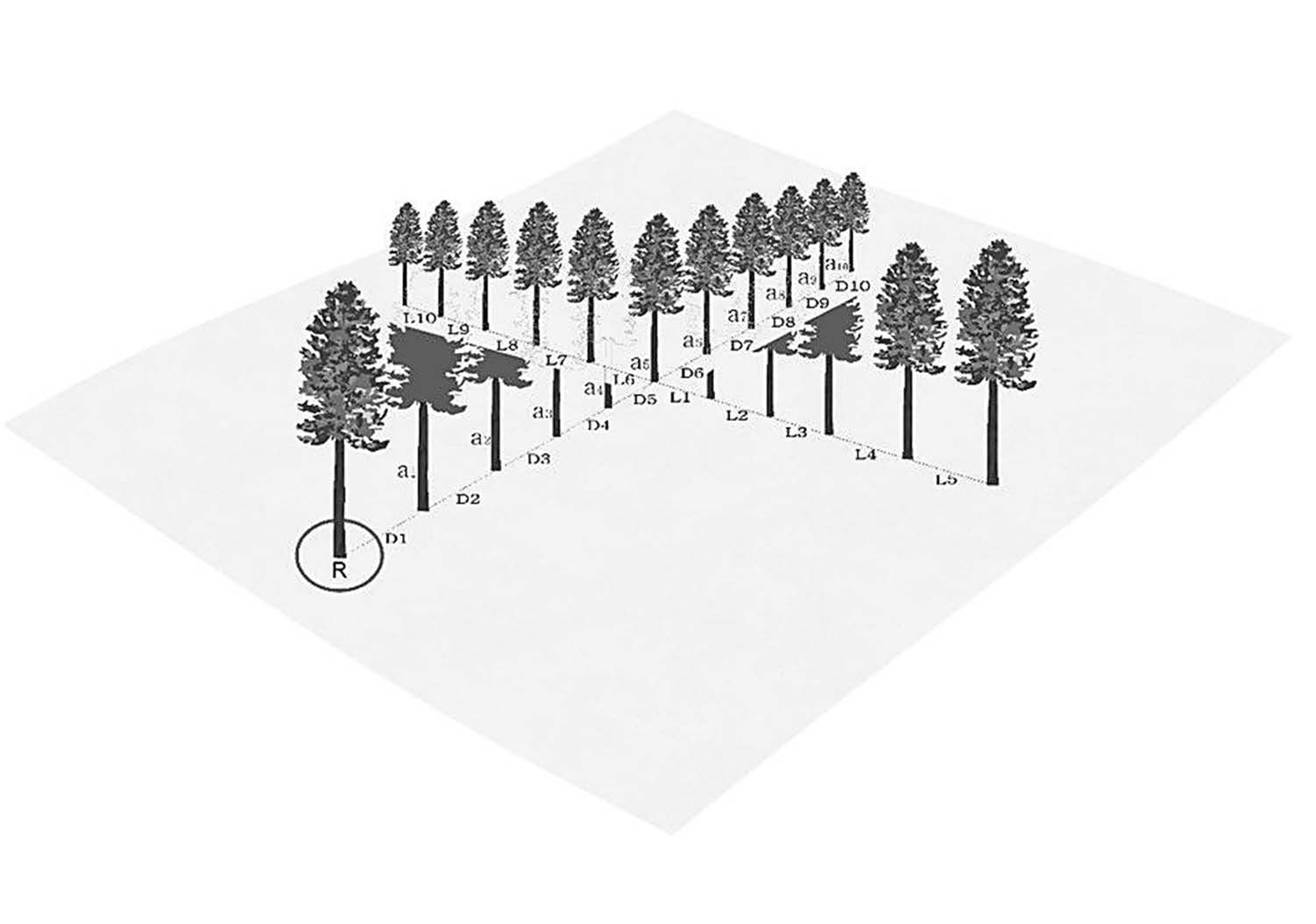
Figure 1 illustrates the proposed sampling unit, in which each tree included was selected with a probability proportional to a geometrical average area per tree, calculated as the product of the mean distances between trees within the row and between rows.

Considering the distances between trees in the row (D_i) and between rows (L_i), the geometrical average area of occupation is calculated by multiplying the means of these distances. This yields m sample area variations (s_i). The overall average area is then obtained by multiplying the respective average distances, which corresponds to the geometric mean of the m separately sampled areas, as defined by Spiegel (¹⁹⁷²).

Figure 1.
Sample unit using the PPGA method.

Probabilistic selection criteria for trees

The probabilistic criterion for tree selection within the sample unit is based on a probability proportional to the geometrical average area of tree occupation within the plot (PPGA). The procedure for defining the sampling unit is described in the following steps:

Select a random geographical coordinate within the stand.
Identify the closest tree to this geographical point to serve as the starting point of the sampling unit, referred to as the reference tree. However, the reference tree will not be included as a measured tree in the sample unit.
From the reference tree, move to the m-th tree along the sample line. The most appropriate number of trees (m) to include in the sampling unit is determined experimentally, based on stabilizing the coefficient of variation for volume per tree as a function of the number of trees in the row.
Measure the distance between the reference tree and the first selected tree (D1) and repeat these measurements sequentially for each tree until the m-th tree is included in the sample unit.
As a result, the sampling unit will consist of a planting row with m trees, starting from the reference tree. If forked trees below 1.30 m are encountered along the sampling row, these additional trees per planting pit will be considered part of the total m trees in the sampling unit.
From the position of the (m/2)-th tree in the row, move perpendicularly to measure the distances (Li) between the j parallel lines on either side of the row (position m/2 on each side) to detect spatial variations within the stand. If forked trees are present, the starting point for this second part of the sampling can be adjusted accordingly .

Defining the probability of inclusion of trees as pi, it can be calculated using (Equation 1):

p_{i} = \frac{\frac{\sum_{i - 1}^{m} D_{i}}{m} \frac{\sum_{i - 1}^{m} L_{i}}{m}}{A} = \frac{\sum_{i = 1}^{m} D_{i} \sum_{i = 1}^{m} L_{i}}{m^{2} A} = \frac{{\overline{D}}_{i} {\overline{L}}_{i}}{A} = \frac{{\overline{E}}_{i}}{A} (1)

(1)

Where: p_i is the mean probability of inclusion of a tree in each sampling unit, Di is the distance between trees in the sampling row, Li is the distance between the planting rows, A is the area of the population to be sampled, and is the average geometric area of occupation of the trees in each sampling unit, m is the number of trees in the row in each sampling unit. The value of m is fixed for the proposed sampling structure.

As can be observed, varies from plot to plot, which characterizes the method as a PPS sampling. The inverse of this probability (pi) allows for an unbiased estimate of the number of trees per hectare, as shown in (Equation 2):

\frac{1}{p_{i}} = p_{i}^{- 1} = \frac{A}{{\overline{E}}_{i}} (2)

(2)

In this sampling procedure, a dichotomous condition occurs, using a categorical variable Zi, i.e., (Zi = 1) when the tree participates in the sampling unit, and (Zi = 0) otherwise. The sampling unit is represented by the geometrical average area per tree that each sampled tree occupies in the sampling space of the plot. Considering this geometrical average area, we have a constant value for the m trees sampled in the plot, then the expected values will be taken as a function of this specific area. Therefore, if one specific value of the geometrical average values is associated with one plot, then for the total number of the trees in the forest, (M – 1) values remains unmeasured in the sampled area.

Consequently, the mathematical expectation for the total number of trees per hectare (M) can be expressed as in (Equation 3):

E (\sum_{i = 1}^{M} X_{i}) = \sum_{i = 1}^{M 1} [(Z_{i} = 0) p_{i}^{1}] + \sum_{i = 1}^{1} [(Z_{i} = 1) p_{i}^{1}] = p_{i}^{1} (3)

(3)

Where Xi is a random variable.

By substituting (Equation 2) into (Equation 3), we obtain:

E (\sum_{i = 1}^{M} X_{i}) = p_{i}^{1} = \frac{A m^{2}}{\sum_{i = 1}^{m} D_{i} \sum_{i = 1}^{m} L_{i}} = \frac{A}{{\overline{E}}_{i}} (4)

(4)

Replacing A (the area of one hectare) in (Equation 4), we obtain the estimator expressed per hectare:

N_{i} = \frac{10, 000 m^{2}}{\sum_{i = 1}^{m} D_{i} \sum_{i = 1}^{m} L_{i}} = \frac{10, 000}{{\overline{E}}_{i}} (5)

(5)

Since this estimation is obtained per plot, and if n plots are measured in the stand, the arithmetic mean of the number of trees per hectare (N) in the stand is given by:

N = \frac{\sum_{i = 1}^{n} N_{i}}{n} (6)

(6)

To derive the estimators for basal area and volume, it is necessary to establish the mathematical expectations as a function of the geometrical average area within the plot, calculated using measurements of m distances between the rows of the plantation.

The mathematical expectations for these two variables follow a similar approach, using their respective average estimators.

The basal area is obtained by calculating the mean of the cross-sectional areas of the sampled trees within the plot.

{\overline{g}}_{i} = \frac{\sum_{i = 1}^{m} g_{i}}{m} (7)

(7)

Considering the total forest area , the mathematical expectation for the basal area will be obtained as follows:

E (\sum_{i = 1}^{M} g_{i}) = \sum_{i = 1}^{M - 1} ({\overline{g}}_{i} (Z_{i} = 0) p_{i}^{- 1}) + \sum_{i = 1}^{1} ({\overline{g}}_{i} (Z_{i} = 1) p_{i}^{- 1}) (8)

E (\sum_{i = 1}^{M} g_{i}) = \sum_{i = 1}^{1} {\overline{g}}_{i} p_{i}^{- 1} = {\overline{g}}_{i} p_{i}^{- 1}

(8)

Substituting (Equation 4) into (Equation 8), we have:

E (\sum_{i = 1}^{M} g_{i}) = {\overline{g}}_{i} p_{i}^{- 1} = {\overline{g}}_{i} \frac{10, 000 m^{2}}{\sum_{i = 1}^{m} D_{i} \sum_{i = 1}^{m} L_{i}} = 10, 000 \frac{{\overline{g}}_{i}}{{\overline{E}}_{i}} (9)

(9)

Substituting (7) into (9) yields the basal area estimator, as follows:

E (\sum_{i = 1}^{M} g_{i}) = {\hat{G}}_{i} = 10, 000 m^{2} \frac{{\overline{g}}_{i}}{\sum_{i = 1}^{m} D_{i} \sum_{i = 1}^{m} L_{i}} = \frac{10, 000}{m} \frac{\sum_{i = 1}^{m} g_{i}}{{\overline{E}}_{i}} = {\hat{G}}_{i} = 10, 000 \frac{\sum_{i = 1}^{m} g_{i}}{m {\overline{E}}_{i}} (10)

(10)

The arithmetic mean of the basal area for the entire stand () is obtained for n sampled units as follows:

\hat{G} = \frac{\sum_{i = 1}^{n} {\hat{G}}_{i}}{n} (11)

(11)

The mathematical expectation of the volume is calculated as the average of the volumes of all trees sampled within the plot, as follows:

{\overline{v}}_{i} = \frac{\sum_{i = 1}^{m} v_{i}}{m} (12)

(12)

The mathematical expectation of the total volume in the stand is obtained as follows:

E (\sum_{i = 1}^{M}) = E (M \overline{v}) = E (M \overline{v}) = M \frac{\sum_{i = 1}^{M} v_{i}}{M} = V (13)

E (\sum_{i - 1}^{M} v_{i}) = \sum_{i - 1}^{M - 1} {\overline{v}}_{i} (Z = 0) p_{i}^{- 1} + \sum_{i - 1}^{1} ({\overline{v}}_{i} (Z_{i} = 1) p_{i}^{- 1})

E (\sum_{i = 1}^{M} {\overline{v}}_{i}) = \sum_{i = 1}^{1} {\overline{v}}_{i} p_{i}^{- 1} = {\overline{v}}_{i} p_{i}^{- 1}

(13)

By substituting (Equation 12) into (Equation 13) and applying the identities for the probability p_i⁻¹ as previously done to estimate the basal area, we obtain:

E (\sum_{i = 1}^{M} v_{i}) = {\overline{v}}_{i} p_{i}^{- 1} = \overline{v} \frac{10, 000 m^{2}}{\sum_{i = 1}^{m} D_{i} \sum_{i = 1}^{m} L_{i}} = 10, 000 \frac{\overline{v}}{{\overline{E}}_{i}} = 10, 000 \frac{\sum_{i = 1}^{m} v_{i}}{m {\overline{E}}_{i}} (14)

V_{i} = 10, 000 \frac{\sum_{i = 1}^{m} v_{i}}{m {\overline{E}}_{i}}

(14)

The arithmetic mean of volume per hectare for the entire stand (V) is obtained for n sampled units as follows:

V = \frac{\sum_{i = 1}^{n} V_{i}}{n} (15)

(15)

To facilitate the application of this sampling method, a function called PPGA was developed to process the sample data using the Julia programming language and is included as part of this work.

Experiment in Pine Forest Stands

This research was conducted in Pinus taeda stands at Pontilhão Farm, owned by FComp, located in São Mateus do Sul, Paraná, Brazil, near the coordinates 50°35›27.07»W and 25°55›36.29»S (^{IBGE, 2006}).

The stands were planted with a spacing of 2.0 m x 2.5 m, resulting in an initial density of 2,000 trees per hectare. The experiment compared estimates of density, basal area, and volume obtained using the PPGA method with those from the conventional forest inventory (IFCON), which employed simple random sampling with plots distributed across three stand management regimes.

The management regimes were characterized as follows:

(i) Regime 1: 12 years old, planted from seeds in July 2005, with a spacing of 2.0 m x 2.5 m, and no thinning.

(ii) Regime 2: 13 years old, planted from seeds in 2004, with a spacing of 2.0 m x 2.5 m, and one thinning (a mixed system: systematic thinning every fifth row and selective thinning in the remaining rows).

(iii) Regime 3: 24 years old, planted from seeds in 1993, with a spacing of 2.0 m x 2.5 m, and selective thinning at 8, 14, 17, and 20 years of age.

In each management regime, several plots were randomly selected, and the sample units of the PPGA sampling method were allocated independently of the fixed-area permanent plots that are part of the company’s continuous forest inventory (CFI). The number of sample units allocated in both experiments is presented in Table 1.

Thumbnail

Table 1.
Number of experimental units allocated in the stands by management regime in Pinus taeda stands.

In these sample units, the measured variables included circumference at breast height (cm), total height (m), and the tree count per plot. Circumference was measured using a metric diameter tape, and height was measured with a Vertex hypsometer.

Using the plot data, the cross-sectional area of each tree and the basal area per hectare were calculated based on the method’s estimators. Tree stem volume was determined by integrating Schöpfer’s fifth-degree taper function ( , , , , , and ) with coefficients adjusted for the experimental area, achieving an R² of 98.63%.

In the PPGA method, distances between trees within sample rows and between rows were measured using a 50-m measuring tape. The fixed-area method utilized circular permanent plots of 900 m². Mean estimates and variances for both methods were calculated and are presented in the results.

Estimates of density (N, number of trees per hectare), basal area (G, m².ha⁻¹), and volume (V, m³.ha⁻¹) were obtained for both methods. Comparisons were conducted to test the hypothesis that the means, variances, and covariances of the estimators do not differ statistically between the two sampling methods.

The null hypothesis for the means of the variables was tested simultaneously using the Hotelling T2 test for two independent vectors. The tests were conducted at a 95% confidence level and are described in Johnson & Wichern (¹⁹⁸⁸).

PPGA Simulation in an Experiment with a Eucalyptus Clone

The PPGA method was applied to a 20.79-hectare eucalyptus stand as part of a forest census. The study area, located between coordinates -46º48’ and -5º51’ (WGS84), consists of a clonal Eucalyptus sp. plantation aged 4.5 to 5 years, in Maranhão, Brazil.

For each living tree, diameter at breast height (cm), tree height (m), and inter-tree distances (m) were measured. These data were mapped using ArcGIS software. Tree volumes were estimated using the Schumacher-Hall nonlinear volumetric function, developed specifically for the study area (Equation 16). The equation was applied to all measured trees, yielding the census volume and the parametric mean (𝜇) of volume stock per hectare.

{\hat{v}}_{i} = 0.000044487 d_{i}^{1.737148116} h_{i}^{1.17608127} (16)

(17)

where: is the predicted tree volume, in m³, is the diameter measured at 1.30 meters aboveground, in cm, and is tree total height, in m.

PPGA plots were randomly distributed across two sampling intensities. The first, n6, consisted of one plot per 4 hectares, totaling six plots. The second, n11, consisted of one plot per 2 hectares, totaling 11 plots. ArcGIS software was used to map the PPGA sampling units and collect volume data () for each of the 10 trees, as well as the distances between trees within a row (Di) and between rows (Li).

This procedure was repeated 100 times for each sampling intensity (n6 and n11). Using these data, the mean and confidence interval of the volume stock (m³ha⁻¹) were calculated and compared with the parametric mean volume (m³ha^-1).

The evaluation of the coefficient of variation of volume per tree as a function of the number of trees in the PPGA method was conducted using a random sampling of 100 plots.

RESULTS

Experiment in Pine Forest Stands

As shown in Figure 1, each tree in the sampling unit was selected with probability proportional to the geometrical average area of occupation. Variations of these geometrical average areas for the plots in the sampled forest stands are presented in Table 2.

Thumbnail

Table 2.
Results of the PPGA sampling method by plot, stand, and management regime.

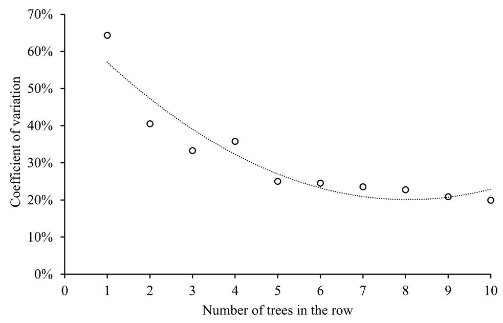
The optimal number of trees for the sampling unit was determined through successive experimental evaluations of the volume coefficients of variation per plot, gradually increasing the number of trees in the sampling unit. The results for different management regimes are shown in Figure 2. As observed, stabilization of the coefficients of variation occurred when m reached 10 trees, indicating that this number is sufficient for the sampling unit.

Figure 2.
Coefficient of variation of volume per tree as a function of the number of trees in the plots of the PPGA method across management regimes in Pinus taeda stands.

In the method proposed by Cottam & Curtis (¹⁹⁵⁶), using only one tree per subunit in the cluster would be insufficient for accurate basal area and volume estimates, as the coefficient of variation would be too high. This method was originally designed for sampling species variation in ecological studies, which limits its applicability for this purpose.

In Prodan’s method, an evaluation was conducted by increasing the number of trees at the sampling point. He proposed including six trees after observing the stabilization of the coefficient of variation in volume estimates.

The results presented in Table 3 show the estimated values for the number of trees, basal area, and volume per hectare in the plots allocated within Pinus taeda stands using the PPGA sampling method. These results were compared with those obtained from the permanent sample plots of the continuous forest inventory. Sampling was conducted in plots where thinning had already been performed, in stands where thinning had not yet been carried out, and in stands that had undergone multiple thinning procedures.

Thumbnail

Table 3.
Average results of the PPGA sampling method and the fixed-area method with circular plots.

Evidence supported the acceptance of the null hypothesis for all three scenarios in which the experiment was conducted. This indicates that the values estimated in the CFI for the variables N, G, and V did not differ between the sampling methods (Table 4).

Thumbnail

Table 4.
Results of the Hotelling T² test comparing the PPGA sampling method with the fixed-area method using circular plots at a 95% confidence level

Here, p is the number of variables, n₁ is the number of observations for the variables in the PPGA method, and n₂ is the number of observations for the variables in the traditional method (fixed-area plot)

PPGA simulation in an experiment with a eucalyptus clone

Seven trees were sufficient to stabilize the coefficient of variation for tree volume, indicating that the sample unit size was adequate to capture the variation among trees for the tested species (Figure 3). This demonstrates the practicality of the PPGA plot in optimizing sampling effort and resources while ensuring data representativeness and result reliability, particularly for volume estimation—a critical variable in forest management decision-making.

Figure 3.
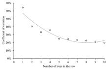
Coefficient of variation of volume per tree as a function of the number of trees in 100 plots using the PPGA method in Eucalyptus stands.

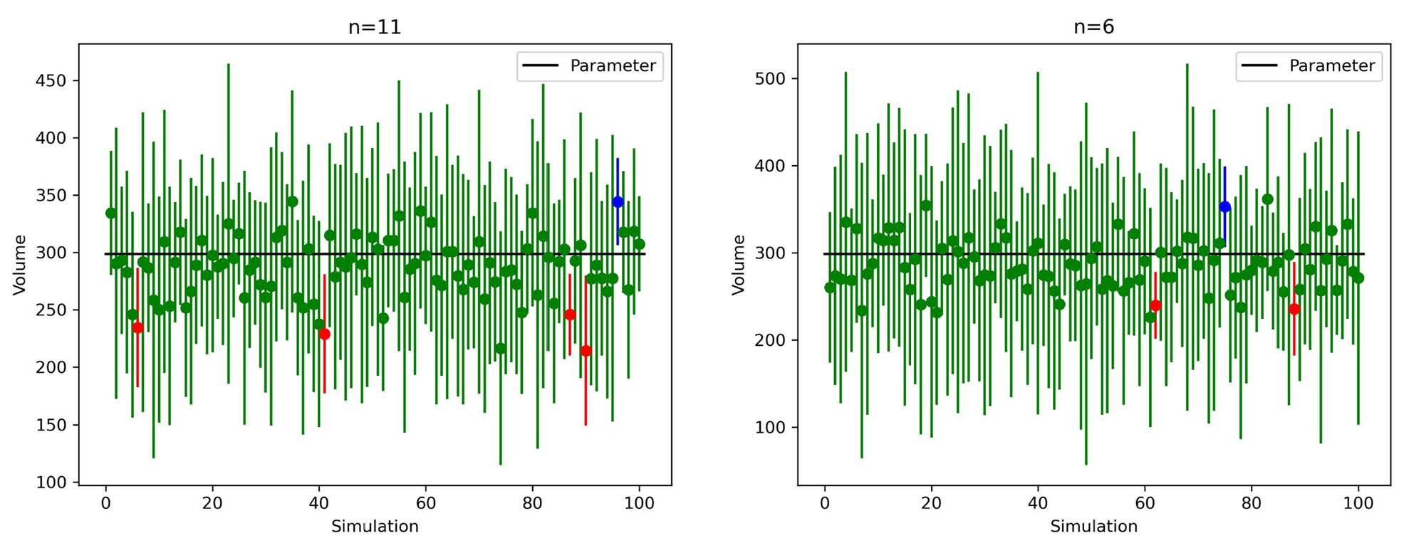
The simulation conducted for the two sampling intensities (n6 and n11), with 100 replications each, revealed that at least 95% of the time, the confidence interval included the mean volume (m³ha⁻¹), along with the estimated mean () approaching the parameter (μ) (Figure 4). The average k deviations was -12.49 m³ha^-1 (-4.18%) for the sample size n6 and -12.51 m³ha^-1 (-4.19%) for the sample size n11, revealing consistent results.

The increase in sampling intensity resulted in narrower confidence intervals, demonstrating more efficient results-a trend commonly observed in such simulation studies. The findings indicated that both sampling intensities provided consistent and reliable estimates of wood volume (m³ha⁻¹), with acceptable variations relative to the parametric mean across the 100 repetitions of the sampling process.

The high coverage of the confidence intervals highlights the robustness of the sampling method, ensuring that most estimates are close to the parametric mean. Additionally, the results of the average deviations for the two sampling intensities suggest excellent sampling accuracy and coverage.

Figure 4.
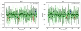
Confidence intervals for the average volume (m³ha⁻¹) obtained from 100 simulations in Eucalyptus stands.

DISCUSSION

The application of the PPGA sampling method proved to be appropriate and consistent for estimating tree density, basal area, and volume per hectare. When compared with results from the conventional forest inventory using fixed-area plots, the average per hectare estimates showed no statistical differences, thereby confirming the formulated hypothesis.

As noted in the introduction, overestimation issues commonly arise, particularly in Prodan’s method, where trees are selected with probabilities proportional to the square of the distance between a point and a tree. Since these distances do not correspond to a biological variable, sample estimates become inversely proportional to the square of these distances. Consequently, the calculated spatial occupation areas are smaller than those derived from measuring distances between trees, resulting in overestimated sampling values.

In this study, the use of biological distances—measured as distances between trees was proposed. This approach ensures more consistent calculations of spatial occupation and allows for a more realistic evaluation of population density. The increase in the calculated area based on these tree distances effectively addresses the overestimation problem.

The geometric mean of distances was found to be an appropriate method for determining the average spatial occupation of trees in each plot within the stand. This approach enabled the derivation of mathematical expectations for the estimators tailored to the specific conditions of the population, accommodating variations in stand characteristics, ages, and management regimes.

As discussed by Péllico Netto (¹⁹⁹⁴), the issue of half-trees, considered marginal trees in Prodan’s method, is entirely resolved in the PPGA sampling method. This is because the structure of the sample unit in the PPGA method does not permit the existence of marginal trees. This characteristic significantly enhances the consistency of the estimators proposed in the new method.

As highlighted by Buck et al. (²⁰¹⁷), the application of Terrestrial Laser Scanning (TLS) in forest inventory practices, particularly when integrated with new technologies for measuring trees in a sample, revealed challenges due to shading effects. These effects often hinder the ability to obtain complete sampling results.

To address this issue, we proposed the PPGA sampling method, which offers practicality and operational ease in the field. The method aims to adapt TLS as a new procedure for generating estimates of parameters that characterize forest populations. By sampling along a line within the stand, the PPGA method minimizes tree occlusions and requires only two scans at the ends of the sample unit—one at the beginning and one at the end, on opposite sides of the sampled row.

Considering that small sample units, such as those used in the PPGA method, are cost-effective in continuous forest inventories (CFIs), a composition of four PPGA subunits arranged in a linear cluster could be established as a permanent plot. This arrangement would enable the identification of the heights of dominant trees, which is essential for monitoring site index diversity within stands. Additionally, in this configuration, each dead tree in a subunit can be replaced by a new tree during successive remeasurements, unlike in fixed-area plots.

In continuous inventories of fixed-area permanent plots, the number of trees tends to decrease over time due to natural mortality or management interventions. The PPGA approach proposes adding new trees in subsequent remeasurements, even under these conditions. Experimental results will determine which of the two approaches increases the autocorrelation between measurements.

In continuous inventories of fixed-area permanent plots, the number of trees tends to decrease over time due to natural mortality or management interventions. The PPGA approach proposes adding new trees in subsequent remeasurements, even under these conditions. We expect that the correlation with the PPGA structure will increase, but only experimental results will determine which of the two approaches increases the autocorrelation between measurements.

The PPGA approach maintains a consistent number of trees per subunit, ensuring greater correlation of volume per cluster across successive measurements compared to fixed plots. This consistency is highly desirable as it reduces covariance in growth precision calculations between successive evaluations. If PPGA clusters are used as permanent sample plots, a new hypothesis could be tested: employing more small plots instead of fewer larger fixed plots, without increasing costs, could enhance the detection of site index variability within stands.

In the present study area with Eucalyptus plantations, circular plots typically range in size from 200 m² to 400 m², with sampling intensities varying from 1 plot per hectare to 1 plot per 10 hectares. It is important to emphasize the practicality of plot allocation and measurement. A PPGA plot requires, on average, 5 minutes to install and measure, compared to approximately 40 minutes for a 400 m² circular plot. This efficiency allows for a higher number of PPGA plots to be installed per unit area.

The practicality of the PPGA method, demonstrated by its quick installation and measurement process, coupled with its accurate volume estimator, makes it highly appealing to forest inventory professionals. Furthermore, the higher sampling intensity achievable with PPGA plots enables a more detailed assessment of variations in the sampled variables. This is particularly beneficial for forest management, especially in detecting site index variability with greater spatial precision.

CONCLUSION

The PPGA sampling method demonstrates consistency across various plot conditions, stand ages, and management regimes in Pinus taeda and Eucalyptus plantations. Estimates for N, G, and V obtained using this method are statistically aligned with those from the company’s permanent plots and with the parametric volume for Eucalyptus forest stands.

The number of 10 trees in the row, distance between trees in the sampling row and 10 distance between the planting rows per PPGA plot was appropriate for the proposed sampling structure.

The method’s use of biological distances between trees prevents overestimation, providing a consistent and suitable approach. By employing the geometric mean of distances, it effectively determines the average spatial domain, ensuring reliable estimations across diverse stand conditions.

The PPGA method is practical, cost-effective, and compatible with the use of TLS, simplifying fieldwork by requiring only two scans at opposite ends of the sampling unit. Its fixed number of trees per plot yields results comparable to those of fixed-area plots, making it a viable and efficient option for continuous forest inventory.

REFERENCES

^1. Assmann E. The principles of forest yield study. New York: Pergamon; 1970.
^2. Bitterlich W. Die Winkelzählprobe. Allgemeine Forst-und Holzwirtschaftliche Zeitung 1948; 59: 4-5.
^3. Buck ALB, Lingnau C, Machado ÁML, Péllico, S. Detecção de árvores em nuvens de pontos de varredura laser terrestre. Boletim de Ciências Geodésicas 2017;23(1):21-38.
^4. Cottam G, Curtis JT. The use of distance measures in phytosociological sampling. Ecology 1956;37(3):451-460.
^5. De Vries PG. Sampling theory for forest inventory: a teach-yourself course. New York: Spring Verlag; 1986.
^6. Instituto Brasileiro de Geografia e Estatística – IBGE. SIRGAS2000: O Referencial Geocêntrico do Brasil. Ponto de Referência 2006; 1:1-28.
^7. Johnson RA, Wichern DW. Applied multivariate statistical analysis. New Jersey: Prentice-Hall; 1988.
^8. Péllico Netto S. Fator de correção para árvores marginais em métodos de amostragem com seleção probabilística proporcional a um tamanho. Revista Cerne 1994;1(1):73-77.
^9. Péllico Netto S, Brena DA. Inventário Florestal. Editado pelos autores, Curitiba, Brasil; 1997.
^10. Péllico Netto S, Stefanello FR, Pellissari AL, David HC. Mapping of sites in Forest stands. Anais da Academia Brasileira de Ciências 2014; 86(4):2025-2037.
^11. Prodan M. Punktstichprobe für die forsteinrichtung. Der Forst-und Holzwirt 1968; 23(11):225-226.
^12. Schöepfer W. Automatisierung dês massen, sorten und wertberechung stender waldbestande schriftenreihe bad. Berlin:Wurtt-Forstl 1966.
^13. Smaltschinski T. Bestandesdichte und verteilungsstruktur. [Dissertation]. Universität Freiburg, Deutschland; 1981.
^14. Stefanello FR Mapeamento de sítios com uso de amostragem sistemática. [Dissertação]. Universidade Federal do Paraná, Brazil; 1994.
^15. Strand L. Sampling for volume along a line. Medd Nor Skogforsok 1958;51(11):327-331.
^16. Spiegel MR. Theory and problems of statistics. McGraw-Hill, Rio de Janeiro, Brazil; 1972.

Edited by

Associate editor:
Emanuel José Gomes de Araújo

Publication Dates

Publication in this collection
17 Mar 2025
Date of issue
2025

History

Received
01 Dec 2024
Accepted
01 Feb 2025

Creative Commons License. All the contents of this journal, except where otherwise noted, is licensed under a Creative Commons Attribution License

[1] ^1. Assmann E. The principles of forest yield study. New York: Pergamon; 1970.

[2] ^2. Bitterlich W. Die Winkelzählprobe. Allgemeine Forst-und Holzwirtschaftliche Zeitung 1948; 59: 4-5.

[3] ^3. Buck ALB, Lingnau C, Machado ÁML, Péllico, S. Detecção de árvores em nuvens de pontos de varredura laser terrestre. Boletim de Ciências Geodésicas 2017;23(1):21-38.

[4] ^4. Cottam G, Curtis JT. The use of distance measures in phytosociological sampling. Ecology 1956;37(3):451-460.

[5] ^5. De Vries PG. Sampling theory for forest inventory: a teach-yourself course. New York: Spring Verlag; 1986.

[6] ^6. Instituto Brasileiro de Geografia e Estatística – IBGE. SIRGAS2000: O Referencial Geocêntrico do Brasil. Ponto de Referência 2006; 1:1-28.

[7] ^7. Johnson RA, Wichern DW. Applied multivariate statistical analysis. New Jersey: Prentice-Hall; 1988.

[8] ^8. Péllico Netto S. Fator de correção para árvores marginais em métodos de amostragem com seleção probabilística proporcional a um tamanho. Revista Cerne 1994;1(1):73-77.

[9] ^9. Péllico Netto S, Brena DA. Inventário Florestal. Editado pelos autores, Curitiba, Brasil; 1997.

[10] ^10. Péllico Netto S, Stefanello FR, Pellissari AL, David HC. Mapping of sites in Forest stands. Anais da Academia Brasileira de Ciências 2014; 86(4):2025-2037.

[11] ^11. Prodan M. Punktstichprobe für die forsteinrichtung. Der Forst-und Holzwirt 1968; 23(11):225-226.

[12] ^12. Schöepfer W. Automatisierung dês massen, sorten und wertberechung stender waldbestande schriftenreihe bad. Berlin:Wurtt-Forstl 1966.

[13] ^13. Smaltschinski T. Bestandesdichte und verteilungsstruktur. [Dissertation]. Universität Freiburg, Deutschland; 1981.

[14] ^14. Stefanello FR Mapeamento de sítios com uso de amostragem sistemática. [Dissertação]. Universidade Federal do Paraná, Brazil; 1994.

[15] ^15. Strand L. Sampling for volume along a line. Medd Nor Skogforsok 1958;51(11):327-331.

[16] ^16. Spiegel MR. Theory and problems of statistics. McGraw-Hill, Rio de Janeiro, Brazil; 1972.

Condition	Plot - nº	E _i	N / ha	G (m²ha ^-1 )	V (m³ha ^-1 )
One thinning	1	12.36	809	42.05	330.79
	2	12.33	811	32.12	235.16
	3	12.48	801	27.44	220.73
	4	11.63	860	36.26	304.22
	5	12.10	826	32.02	270.78
	6	13.09	764	26.71	223.97
	7	10.64	940	28.87	227.19
	8	9.95	1005	37.73	310.89
	9	10.73	932	39.34	325.93
Without thinning	1	5.50	1818	72.56	640.94
	2	5.84	1713	60.49	529.24
	3	6.42	1557	64.84	508.50
	4	6.80	1471	44.67	339.77
	5	5.59	1790	55.93	456.60
	6	7.26	1377	51.96	437.84
Various thinnings	1	27.83	359	44.94	553.25
	2	106.42	94	22.44	286.37
	3	24.16	414	51.40	660.07

Condition	Method / Variable
	PPGA	Circular Plot
	N (ha)
One thinning	861	784
Without thinning	1581	1585
Various thinning	387	385
	G (m².ha ^-1 )
One thinning	33.61	29.90
Without thinning	55.58	52.30
Various thinning	48.17	46.40
	V (m³.ha ^-1 )
One thinning	272.19	254.43
Without thinning	545.27	463.62
Various thinnings	727.99	699.90

Condition	T² calculated		Conclusion
One thinning	3.15	3.49	Not significant
Without thinning	2.69	4.75	Not significant
Various thinning	0.19	6.59	Not significant

Management regime	PPGA	Fixed area sampling
Regime 1	6	5
Regime 2	9	7
Regime 3	3	6
Total	18	18