Structural persistence of Brazil’s inflation rate in times of fiscal bubbles^♦

Persistência estrutural da inflação brasileira em regime de bolhas fiscais

Abstract

We estimate the hybrid Phillips curve to verify whether the explosive debt bubble regime can affect inflation’s level and persistence as measured by the IPCA price inflation from January 2002 to November 2023. Gross debt-to-GDP ratio explosive behavior significantly increases the weight of backward-looking price-setters, leading to cost push shocks that are more persistent and policy less potent. We find a downward bias in the lagged inflation coefficient in which only a lower fraction of the firms are backward-looking price-setters using the standard approach. More specifically, the weight of past inflation ranges from 0.24 to 0.77 in standard approaches, while accounting for debt bubble’s inertia coefficient increases to 0.99. The fiscal instance in operation partially explains the inflation dynamics at the time. Under normal conditions, inertia tends to decrease and increase as the public debt reaches an explosive path. Worse fiscal stances can considerably reduce the effectiveness of sounder monetary policy actions in accomplishing the target rising inertia. More sustainable fiscal conditions improve the effectiveness of monetary policy in curbing inflation. Our empirical findings are supported by consistent estimation applying instrumental variables regression methods robust to many (possibly weak) instruments in heteroskedastic environments. We deal appropriately with structural breaks and stationarity issues of the variables under study. Nonlinearity tests and structural break tests at an unknown time with endogenous regressors show that the instability of the parameters plays no role in the results.

Keywords:
Phillips curve; Inflation; Inertia; Debt bubbles; Fiscal policy

Resumo

Estimamos uma curva de Phillips híbrida permitindo mudanças ocasionais no coeficiente da inflação passada e no coeficiente da expectativa de inflação, em que as mudanças nos coeficientes estão associadas ao comportamento explosivo e formação de bolhas de dívida pública. Para dados mensais de janeiro de 2002 a novembro de 2023, utilizando o IPCA como medida de inflação, constatamos que a ocorrência de bolhas de dívida pública eleva significativamente o coeficiente da inflação passada, implicando maior perda de produto e menor eficácia da política monetária para atingir a meta de inflação. Constatamos uma subestimação do coeficiente da inflação passada. Em particular, observamos que o coeficiente da inflação passada varia entre 0,24 e 0,77 na literatura padrão, entretanto, tendo-se em conta o comportamento explosivo da dívida pública, o coeficiente aumenta significativamente para 0,99: a condição fiscal explica parcialmente a dinâmica da inflação, caracterizada pela persistência e o nível de inflação. Na ausência de bolhas de dívida pública a inércia é significativamente menor, contribuindo favoravelmente para o alcance das metas de inflação com menor perda de produto e ganhos de credibilidade. Empregamos métodos que são robustos à presença de (múltiplos) instrumentos fracos e heterocedasticidade. Não há indícios de instabilidade nos coeficientes nem erros de especificação. Empregamos pré-testes formais para quebras estruturais e estacionariedade, aspectos frequentemente negligenciados na literatura.

Palavras-chave:
Curva de Phillips; Inflação; Inércia; Bolha de dívida pública; Política fiscal

1. Introduction

This paper uses two decades of data under inflation targeting regime in Brazil to verify whether the coefficients on lagged inflation and inflation expectations for 12 months ahead remain stable when the debt-to-GDP ratio follows an explosive path over the recurring episodes of sovereign government debt bubbles. An increase in the share of forward-looking price setters indicates that the Central Bank’s improvement in communication strategies can bring inflation down more quickly and at a lower output cost. In contrast, an eventual increase in the share of backward-looking price setters prolongs price pressures, lowering the power of monetary policy actions at a higher output and employment costs. The closest studies to our paper are those by Kwon et al. (2009), Reinhart and Rogoff (2010), and Grigoli and Sandri (2024) which suggest that public debt, rather than budget deficit, plays a significant role in determining the level and persistence of inflation in developing countries.¹ The instability of the Phillips curve parameters and its source of breaks are key considerations in our investigation (Boldea and Hall, 2013; Chowdhury and Sarkar, 2016).

The main findings of the paper are as follows. First, the weight of past inflation ranges from 0.24 to 0.77 in standard approaches. However, adjusting for the effects of the debt bubble, the lagged inflation coefficient increases to 0.99. Under a debt bubble regime, the share of the price-setters that set prices based on past inflation rises substantially. Worse fiscal stances can considerably reduce the effectiveness of sound monetary policy actions in achieving targets over time, thereby increasing inertia. This conclusion remains invariant with the fiscal indicator used in the estimations (debt-to-GDP ratio or gross debt-to-GDP ratio). More sustainable fiscal conditions improve the effectiveness of monetary policy in curbing inflation by lowering the inertia component. Second, the study provides modest methodological advice on the dating stamping algorithm of Phillips et al. (2015), initially designed only for the detection of multiple bubbles in univariate time series. It works well and can be used effectively to investigate multivariate economic relations (e.g., inflation and economic activity) to identify and quantify the effect of policy regime changes.

Lastly, we pay special attention to twin issues of structural breaks and stationarity of the main variables, a drawback pointed out by Sachsida (2013), Medeiros et al. (2017) and Chowdhury and Sarkar (2016). Structural break tests show one sudden significant change in inflation expectations with the estimated break date in October 2010, a few months before the policy regime change in the Central Bank’s reaction function (Cortes and Paiva, 2017). In the case of the output gap, the estimated break date is October 2014, which is very close to the fiscal crisis that peaks in 2014-15 (Holland, 2019).² The primary empirical motivation in this paper comes from observing Figure 1 and the associated behavior of Brazil’s sovereign public debt sharp deterioration (Figure 2 below).

Figure 1 shows the evolution of the actual 12-month cumulative inflation, the 12-month ahead inflation expected by the private sector, and the 12-month ahead inflation target. The main empirical finding in Figure 1 is that the actual cumulative inflation level remains above the target for several periods. This wide gap suggests that the private sector tends to expect that the increase in the inflation rate will not tend to reverse in the medium term (Minella et al., 2003; IMF, 2023). Inflation expectations remained above the target at the beginning of the sample around the presidential elections in 2002, along with the 2008-2009 U.S. financial crisis, predominated after 2010 for several years over the Rousseff administration, and at the sample’s end. Cortes and Paiva (2017) provide a complete account of the change in the reaction function of the Central Bank of Brazil during the Rousseff administration.

We interpret sustained periods in which expectations remain above the target as a loss of credibility. Credibility is vital to conducting monetary policy because it helps make disinflation less costly and gain public support for policy actions of the Central Bank (Malikane and Mokoka, 2012; IMF, 2023). Credibility implies that if private sector expectations diverge from targets, we should observe an eventual return (Minella et al., 2003; Lyziak and Paloviita, 2017). Most authors, such as Minella et al. (2003) and, more recently, Malikane and Mokoka (2012) and Cortes and Paiva (2017), emphasize the Central Bank’s behavior and preferences in attaining credibility, ignoring the fiscal stance disarray and its primary effects in changing inflation dynamics. The literature is still silent on this point. However, other approaches exist.

Figure 1
This plot shows the evolution of the actual 12-month cumulative inflation by IPCA (blue), the 12-month ahead inflation expectations (red), and the annual inflation target (magenta), in percentage points, over January 2002 to November 2023 (T=263 observations).

This paper complements the work of Minella et al. (2003), Malikane and Mokoka (2012), Cortes and Paiva (2017) and Lyziak and Paloviita (2017) by examining the role that fiscal stance plays in changing inflation dynamics (e.g., inertia), affecting credibility and price stability (Dornbusch et al. 1990; Erceg and Levin, 2003; Celasun et al., 2004; Bianchi and Melosi, 2022). Dornbusch et al. (1990) agree with Fraga et al. (2004) by claiming that better institutions, such as independent Central Bank, are crucial to building credibility and reaching price stability. However, a government unwilling to balance the budget can undermine credibility, for instance, by generating a public debt bubble (Bruno and Fischer, 1990; Woodford, 2001; Kwon et al., 2009). According to Dornbusch et al. (1990), Dornbusch and Cline (1997), Celasun et al. (2004), Bianchi and Melosi (2022), when building credibility, one needs to pay more attention to fiscal stance behavior and not only to the Central Bank’s monetary policy decisions. In particular, Celasun et al. (2004) empirically show the importance of building fiscal credibility, in which improvements in various measures of fiscal balances significantly reduce inflation expectations.

The empirical findings of the present study suggest that the departure from the target observed in Figure 1 can be statistically associated with the identification of the date of the multiple debt bubbles (Table 2). Furthermore, theory suggests that in a macroeconomic environment of a sharp deterioration of the sovereign public debt, a worse fiscal condition affects the performance of monetary policy under an inflation targeting regime (Woodford, 2001; Reinhart and Rogoff, 2010; Leeper and Leith, 2016). It can increase the risk premia, interest rates, and expected inflation rates, compromising the effectiveness of monetary policy. More specifically, Blanchard and Fischer (1989) and Bruno and Fischer (1990) demonstrate that households and firms can change how they set prices and wages in response to a public debt bubble by putting more weight on past inflation: the slope parameters of a Phillips curve can capture these occasional changes (Galí et al., 2001; Blanchard, 2021; Fuhrer, 2011).

Based on all these considerations, we employ two decades of data under inflation targeting regime in Brazil to determine whether the lagged and expected inflation coefficients remain constant when the debt-to-GDP ratio follows an explosive path over the recurrent episodes of government debt bubbles. The fiscal stance in operation might partially explains the changes in inflation dynamics at that time, significantly increasing inertia. Under normal conditions, inertia tends to decrease and increase as the public debt reaches an explosive path. These regime changes can be empirically estimated. The existing literature studying the instability of the Phillips curve fails to point out the sources of those changes when they are present in the estimates.

In addition, regarding the potential structural breaks in the series, the methods employed allow us to identify the source of the change in inflation dynamics, while previous studies have not. Furthermore, we test for structural changes in the trend function of the series without knowing whether the noise component is stationary or integrated (Perron and Yabu, 2009), which represents some advances in regards to Luengo-Prado et al. (2018) for US data and Medeiros et al. (2017) for Brazilian data.

The paper provides three main contributions to previous studies that estimate the Phillips curve for Brazil. First, departing from Minella et al. (2003), Muinhos (2004), Areosa and Medeiros (2007), Mazali and Divino (2010), and Arruda et al. (2018), which assume constant parameters, we allow for occasional changes in two slopes of the Phillips curve by identifying its sources, associated with recurrent episodes of public debt bubbles, as the theory suggests (Bruno and Fischer, 1990; Blanchard and Fischer, 1989). Second, in contrast to Cati et al. (1999), in which the chosen dates of changes in inertia parameter are given exogenously, we let the data speak for themselves using recursive evolving algorithm proposed by Phillips et al. (2015) and implemented by Vasilopoulos et al. (2022). More specifically, we assume that we do not know exactly when the bubble emerges and its duration over time, and let the data speak for themselves in this regard by consistently estimating the start and end of the bubbles. The simulations performed by Phillips et al. (2015) suggest that the method is fully reliable in detecting multiple bubbles. Finally, the paper pays special attention to the twin issues of structural break and stationarity, an apparent gap in the literature in Brazil (Sachsida, 2013) and worldwide (Chowdhury and Sarkar, 2016). Based on the methods of Perron and Yabu (2009) and Kim and Perron (2009), we find that actual inflation, the output gap, and the expected inflation at 12 months follow a stationary process throughout the period from January 2002 to November 2023, exhibiting transitory fluctuations around a more or less stable trend path.

Two macroeconomic changes in fiscal and monetary conditions observed in Brazil in the 2000s provide context to the present study. First, Holland (2019) detects policy changes in fiscal conditions of the government’s consumption during the 2000s that led to the fiscal collapse peaked in 2014-17. Campos and Cysne (2019) found that the Brazilian public debt reached an unsustainable path in several periods using data from 2003 to 2016. Second, Cortes and Paiva (2017) detect changes in the reaction function of the Central Bank of Brazil at the start year of the first Rousseff administration. According to Zhang et al. (2008), any change in the conduct of monetary policy can change the dynamics of the inflation. The structure of the paper is the following. Section 2 presents the specification models and describes the data used in the estimations. Section 3 discusses and compares the main findings to the literature on prior empirical Phillips curve for Brazil estimates. Section 4 provides brief conclusions.

2. Econometric methodology

2.1. Dating the debt bubbles episodes

Phillips and Shi (2019) apply the evolving date stamping algorithm proposed by Phillips et al. (2015) to identify the increasing sovereign risk in Greece, Ireland, Italy, Portugal and Spain from January 2001 to September 2016, which preceded a high level of public debt. Unlike Phillips and Shi (2019), in which the main objective is exclusively to detect dates of exuberance and collapse embedded in univariate setup, in the present study the main objective is to investigate the role of public debt on the level and persistence of inflation embedded in a multivariate setup guided by economic theory, as suggested in Kwon et al. (2009), Reinhart and Rogoff (2010), Leeper and Leith (2016), and Grigoli and Sandri (2024). Thus, this paper follows the standard approach to represent the fiscal instance of the economy as reflected in the debt-to-GDP ratio (Silva and Medeiros, 2009; Reinhart and Rogoff, 2010; Holland, 2019; Blanchard, 2021; Grigoli and Sandri, 2024) because economic theory suggests greater and significant influence of public debt on determining inflation level and persistence, which is the central focus of the present paper. As there is well-documented empirical evidence from Brazilian data (Grigoli and Sandri, 2024) showing that agents systematically underestimate the public debt level in Brazil when measured by the standard debt-to-GDP ratio, we also use the gross debt-to-GDP ratio, the second most important fiscal indicator according to Silva and Medeiros (2009), to further investigate the likely influence of public debt on inflation level and persistence. In fact, institutions such as IMF (2024) and some researchers, such as Barbosa Filho (2017), when studying the Brazilian economy, consider the government’s gross debt as a percentage of GDP as the main fiscal indicator. In the same direction, Leeper and Leith (2016) has also used the government’s gross debt to GDP as the main fiscal indicator that affects inflation when studying the same issue for the US economy. We left to the data to speak for themselves, which is the most informative fiscal indicator when studying the level of inflation and persistence in Brazil. Silva and Medeiros (2009) provide detailed information on the main concepts of public debt in Brazil, including available statistics and data sources, as well as their application in empirical studies.³

The class of test procedures described in Vasilopoulos et al. (2022) can be applied to identify and date-stamp explosive behavior periods of exuberance in public debt and asset price bubbles (Phillips et al., 2015; Phillips and Shi, 2019).⁴ The method is based on the ADF model specification for fitted regression, along with flexible window widths to consider time-varying dynamics and potential structural breaks. Consider the following ADF regression model:

$\Delta y_t=a_{r\mathrm{1,}r2}+{\gamma }_{r\mathrm{1,}r2}{y}_{t-1}+{\displaystyle \sum }_{j=1}^k{\Psi }_{r\mathrm{1,}r2}^j\Delta y_{t-j}+{\epsilon }_t$ (1)

where $y_t$ represents the ratio of the debt to GDP or the data on the ratio of gross debt to GDP, $\Delta y_t$ with $j=\mathrm{1,}\dots ,k$ are lagged first differences of the series to deal with serial correlation. ${\epsilon }_t$ are the Gaussian residuals, and $a_{r\mathrm{1,}r2},{\gamma }_{r\mathrm{1,}r2},{\Psi }_{r\mathrm{1,}r2}^{j}withj=\mathrm{1,}\dots ,k$ are regression coefficients. The subscripts $r_{1}and{r}_2$ represent fractions of the total sample size T and specify the starting and ending points of a sub-sample period. The generalized SADF (GSADF) statistic used in this paper verifies whether exuberance is present in a sub-sample by comparing the test statistic with the right-tailed critical value of its limit distribution. Data reject the null hypothesis of unit root against the alternative of exuberance (explosive behavior) when the test statistic exceeds the corresponding critical value at the 5% level. Because this method uses only a univariate approach, it does not distinguish between the various potential causes that could lead the public debt to an explosive path, such as geopolitical changes or domestic mismanagement of public debt. An important lesson comes from Bohn (2007). Testing for unit root does not provide any information regarding the fiscal solvency of public debt, because the intertemporal government budget constraint holds under very weak time-series assumptions that are generally satisfied in the data. Recently, D’Erasmo et al. (2016) suggested three empirical approaches that are considered valid to investigate whether a public debt is sustainable or not. The sustainability of public debt is not studied in the present article.⁵

2.2. The hybrid Phillips curve specifications

There are at least two theoretical reasons for choosing the hybrid Phillips curve as a valid tool to examine the effect of recurrent debt bubble episodes on the level and persistence of Brazilian inflation. First, while the traditional Phillips curve is subject to Lucas’ critique, the hybrid Phillips curve is not (Galí et al., 2001; Chowdhury and Sarkar, 2016). Second, the treatment of inflation expectations on the traditional Phillips curve is insufficient to capture the forward-looking behavior of an individual (Chowdhury and Sarkar, 2016; Fuhrer, 2011). In contrast, the hybrid Phillips curve can adequately capture the backward-looking and forward-looking behavior of price-setters (Galí and Gertler, 1999; Galí et al., 2001; Fuhrer, 2011; IMF, 2023). Based on Galí and Gertler (1999), Galí et al. (2001), Fuhrer (2006; 2011) and IMF (2023), the standard structural hybrid Phillips curve is given by

${\pi }_t={\gamma }_b{\pi }_{t-1}+{\gamma }_f{\pi }_{t+12}^e+\lambda x_t+{\nu }_t$ (2)

where ${\pi }_{t-1}$ is the past inflation,${\pi }_{t+12}^e$ is the 12-month ahead expected inflation given the information available up to period t, $x_t$ measures real economic activity, such as the output gap. The error ${\nu }_t$ term encapsulates all the unmeasured or latent factors that affect the inflation rate. The parameter ${\gamma }_b$ measures the importance of backward-looking behavior in current average inflation that comes from the existence of a fraction of monopolistically competitive firms that set prices using a backward-looking rule of thumb. The parameter ${\gamma }_f$ quantifies the importance of forward-looking behavior for price-setters on average current inflation. Lastly, the $\lambda$ parameter measures the influence of the tightness of the labor market on the average current inflation rate. Our methods do not assume “inflation shock” ${\nu }_t$ is white noise. Indeed, in a more general sense, the inflation shock can be heteroskedastic as serially correlated over time.

As explained in the Introduction, we specify an augmented version of the hybrid Phillips curve able to describe policy regime changes based on the assumption that the slopes on lagged and expected inflation may quite well embed expectations of future inflation (Galí et al., 2001; Blanchard, 2021), where occasional parameter instability may reflect a change in how price-setters form expectations under hostile macroeconomic conditions (Blanchard and Fischer, 1989; Bruno and Fischer, 1990). In this direction, IMF (2023) has implemented a dynamic stochastic general equilibrium model with a mix of forward- and backward-learner agents, showing that the output costs of the monetary policy tightening increase with the share of backward-looking learners. Under hostile macroeconomic conditions, backward-learner agents set prices and wages using only more recent and past information (IMF, 2023).

The t-statistic associated with the categorical variable D (defined below) allows testing this assumption. The model to account for fiscal conditions, as measured by the debt-to-GDP ratio when it reaches an explosive time path, is given by

${\pi }_t={\gamma }_b{\pi }_{t-1}+{\gamma }_u\left(D\cdot {\pi }_{t-1}\right)+{\gamma }_f{\pi }_{t+12}^e+{\gamma }_g\left(D\cdot {\pi }_{t+12}^e\right)+\lambda x_t+{\mu }_t$ (3)

where D assumes one if the debt-to-GDP ratio reaches an explosive path and zero otherwise. When the economy experiences a normal condition of public debt management, Eq. (3) collapses to Eq. (2) because $D=0$. We apply the generalized supremum ADF (GSADF) test statistic proposed by Phillips et al. (2015), as described in Vasilopoulos et al. (2022), to consistently estimate these dates. The categorical variable D defined above is commonly applied to identify and measure policy actions (Cati et al., 1999) and the output effects of the currency and balance of payments crises in emerging market economies (Hutchison and Noy, 2005), to account for changes in the slope of the traditional Phillips curve in the US economy (Luengo-Prado et al., 2018).

The focus of the present paper is to identify and measure the explosive path of the public debt impacts on the level and persistence of average inflation that can change the slopes of the hybrid Phillips curve, given by $\frac{\partial {\pi }_t}{\partial {\pi }_{t-1}}\left(D=1\right)={\gamma }_b+{\gamma }_{u}and\frac{\partial {\pi }_t}{\partial {\pi }_{t+12}^e}\left(D=1\right)={\gamma }_f+{\gamma }_g$. Under normal market conditions in which the public debt is under control, represented by $D=0$, we expect structural stability in the two slopes of the Phillips curve, which are expected to be similar in magnitude to previous studies. More specifically, when the public debt does not follow an explosive path, the slopes of the Phillips curve will be given by $\frac{\partial {\pi }_t}{\partial {\pi }_{t-1}}\left(D=0\right)={\gamma }_{b}and\frac{\partial {\pi }_t}{\partial {\pi }_{t+12}^e}\left(D=0\right)={\gamma }_f$. In this setting, the parameters ${\gamma }_{u}and{\gamma }_g$ are termed differential slopes in the standard textbook literature, and the t-statistic tests its statistical significance. In sum, in the present study, the ${\gamma }_{u}and{\gamma }_g$ parameters measure the differential slope associated with public debt’s explosive path that we expect to modify inflation persistence, changing the way agents form inflation expectations to set prices and wages in the economy (Bruno and Fischer, 1990; Galí et al., 2001; Blanchard, 2021).

The model specification in equations (2) and (3) imply the following moment conditions for parameter estimation,

$E_t\left\{\left({\pi }_t-{\gamma }_b{\pi }_{t-1}-{\gamma }_f{\pi }_{t+12}^e-\lambda x_t\right)z_t\right\}$ (4)

$E_t\left\{\left({\pi }_t-{\gamma }_b{\pi }_{t-1}-{\gamma }_u\left(D\cdot {\pi }_{t-1}\right)-{\gamma }_f{\pi }_{t+12}^e-{\gamma }_g\left(D\cdot {\pi }_{t+12}^e\right)-\lambda x_t\right)z_t\right\}$ (5)

where $z_t$ is a vector of variables dated t and earlier. The orthogonality conditions (4) and (5) are the basis for estimating the basic models (2 and 3) by using the two-step generalized method of moments (GMM) estimator introduced by Hansen (1982) and studied in detail by Hayashi (2000).

The GMM estimation method, despite its wide use and generality, is based on two main conditions. Exogeneity of instruments and relevance of instruments. Even when the instruments are exogenous, as indicated by the p-value of the Hansen J test being higher than the significance level, the GMM method can generate an unreliable inference in the presence of low correlation between the instrumental variables and the endogenous regressors (weak instruments). Stock et al. (2002) provide a review of this literature and discuss various issues, including the issue of the weak instruments problem. Maka and Barbosa (2022) show that this problem can be quite relevant when estimating the various strands of the Phillips curve using Brazilian data.

To circumvent the problems associated with weak instruments in GMM/IV methods, which are pretty standard in practice (Dufour et al., 2006; Maka and Barbosa, 2022), we adopt an IV (instrumental variable) estimation approach that is consistent, efficient, and reliable even in the presence of potentially many weak instruments and heteroskedasticity proposed by Hausman et al. (2012). To test for the validity of the instrumental variables, we use the bias corrected J test statistic suggested by Chao et al. (2014), which overcomes the problems of testing for overidentifying restrictions based on Sargan and Hansen J statistic. The bias corrected J test statistic suggested by Chao et al. (2014) is robust to potentially many weak instruments and heteroskedasticity. We also further investigate the influence of the debt bubble by applying the conditional likelihood ratio (CLR) test statistic proposed by Moreira (2003), which presents high power advantages even in the presence of weak instrumental variables.

2.3. Data and descriptive statistics

We chose the Broad Consumer Price Index (IPCA) reported by the National Bureau of Geography and Statistics (IBGE) because it is the main inflation indicator to gauge the inflation targeting regime in Brazil (Bogdanski et al., 2001; Minella et al., 2003). According to Feijó and Ramos (2013), the IPCA inflation index covers a basket of goods relative to families with personal income between 1 and 40 minimum wages. It includes eleven metropolitan areas (Rio de Janeiro, Porto Alegre, Belo Horizonte, Recife, São Paulo, Belém, Fortaleza, Salvador, Curitiba, Brasília, and Goiânia). All inflation data are used in percentage points per month, and all data series come from IPEADATA (www.ipeadata.gov.br) and Central Bank of Brazil (www.bcb.gov.br).⁶ We follow the work of Minella et al. (2003), Cerisola and Gelos (2009), and IMF (2023) using inflation expectations as the Central Bank conducts the survey among financial institutions and consulting firms, reflecting what firms expect for the year-end inflation in current and following years.

Muinhos (2004), Mazali and Divino (2010), and Malikane and Mokoka (2012) estimate Phillips curve using generated regressors by imputing values to unobserved regressors, such as market expectations, from an auxiliary econometric model. Murphy and Topel (2002) have shown that this two-step procedure to impute the values of unobserved regressors can lead to erroneous inference because the sampling error from the first stage contaminates the second stage estimation. The standard asymptotic variance-covariance matrix does not account for this (Pagan, 1984; Murphy and Topel, 2002). Murphy and Topel (2002) report some examples in which the generated regressors overestimate the t-statistic by 60%, leading to false significance. Pagan (1984) gives a more formal and fully econometric treatment of this problem.

This paper departs from Chowdhury and Sarkar (2016) that used realized inflation as if it were inflation expectations and from those authors that employ generated regressors (Muinhos, 2004; Mazali and Divino, 2010) and follows Minella et al. (2003), Cerisola and Gelos (2009), and IMF (2023) to avoid this econometric issue using survey expectations sampled from market participants. Lastly, regarding the measurement of economic activity, based on the works of Clarida et al. (1998), Favero (2002), and Hosseinkouchack and Wolters (2013), we compute the measurement of the output gap by taking the residuals of an Ordinary Least Squares (OLS) regression of the logarithm of the seasonally adjusted industrial production index on a constant, a linear trend, and a quadratic trend. It would only be a valid output measure if it features a determinist quadratic trend.

As Perron and Yabu (2009) explain, a structural break in the trend function is a problem of long horizon data (two decades of monthly data under inflation targeting regime in Brazil) as in the present study, and the noise component may be stationary or have a unit root. The test statistic proposed by Perron and Yabu (2009) is essential in confronting the circular problem involved in stationarity and structural break in empirical investigations. The circular problem means that most conventional structural break tests, such as the Bai and Perron (2003) methods applied to Brazilian data by Medeiros et al. (2017), require prior information on whether the noise component is stationary or has a unit root. However, verifying whether the noise is stationary requires determining whether the series has a structural break.

Perron and Yabu (2009) proposed a solution to this circular problem by recently devising a structural break test to verify the existence of a break in the trend function of a univariate time series without prior knowledge of whether the noise is stationary or has a unit root. The second column of Table 1 presents the results of the Perron and Yabu (2009) structural break test results. According to Kim and Perron (2009) and Perron and Yabu (2009), these results provide safer guidance in choosing between the standard ADF test and the test introduced by Perron and Yabu (2009) in terms of greater power and correct size.⁷

Table 1
Results of the Perron-Yabu test on structural break and the Kim-Perron/ADF test on unit roots - 2002:01-2023:11

Variable	Perron-Yabu structural break test	Kim-Perron/ADF unit root test
1. Monthly IPCA inflation rate (%)	0.7028	-4.8159**
2. 12-month ahead inflation expectations	12.7331** ($\widehat{TB}=2010:10$)	-3.1736*
3. Output gap	49.5172** ($\widehat{TB}=2014:10$)	-4.2461**

• Notes: (**), (*) denote statistical significance at the 5% and 10% levels, respectively. We apply model I of Perron and Yabu (2009), which tests a change in the series level for the actual inflation series, the 12-month ahead inflation expectations, and the output gap for the Perron-Yabu test. The null hypothesis of the Perron-Yabu test is that the series has no structural break. The reported test statistic uses a trimming percentage of 0.15. The critical values at the 5% and 10% levels are 1.74 and 1.26 for the Perron-Yabu test statistic (Perron and Yabu, 2009, Table 1), respectively. The null hypothesis for the Kim-Perron unit root test is that the series has a unit root. The critical values at the 5% and 10% levels for the Kim-Perron unit root test are -4.24 and -3.96 (Perron, 1989, Table VI.B), respectively. The null hypothesis for the ADF unit root test is that the series has a unit root. The critical values for the ADF unit root test at the 5% and 10% levels are -3.41 and -3.12 (Banerjee et al., 1993, Table 4.2), respectively.

In a recent survey on inflation expectations using Brazilian data, Cambara et al. (2022) tested whether inflation expectations for the next 12 months follow a unit root or are a stationary process applying the standard ADF test from December 2001 to August 2018. The authors do not reject null hypothesis of the unit root for inflation expectations. The drawback of this conclusion is that it ignores the potential breaks in the series, which can generate incorrect inferences (Perron, 1989; Perron and Yabu, 2009). In contrast, the findings presented in Table 1 point to a firm rejection of the null hypothesis that the trend function of the inflation expectations and output gap is stable over decades. The last column of Table 1 shows that the data reject unit root for inflation expectations, the output gap, and the series of actual inflation over 2002:01 - 2023:11.

More specifically, the empirical evidence reported in the second column of Table 1 indicates that the trend function of actual inflation in Brazil does not contain a structural break. Thus, in this case, the standard ADF unit root test is the most suitable test to detect the integration order of IPCA price inflation (Kim and Perron, 2009).

However, the same column of Table 1 shows a significant structural break in the deterministic trend in inflation expectations and the output gap. Then, for these two variables, the Kim-Perron unit root test, rather than the standard ADF test, allowing for a structural break under the null and alternative, is the most suitable test to detect the integration order of these series (Kim and Perron, 2009). Overall, as the last column of Table 1 suggests, we can consider the main variables of interest stationary for our GMM/IV estimation procedures.

3. Results and discussion

3.1. GSADF statistic results

Figure 2 shows that both indicators of public debt strongly changed their path a few months before 2015. An upward trend after 2015 replaced a previous downward trend in both fiscal indicators, showing a sudden change in the fiscal conditions of Brazil.

Figure 2
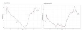
This plot shows the debt-to-GDP ratio in the left panel and the gross debt-to-GDP ratio in the right panel over the period from January 2002 to November 2023 (T=263 observations).

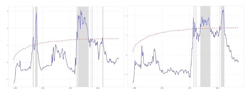
Figure 3 below reveals that once the explosive behavior starts, the GSADF test statistic (in blue) smoothly increases and exceeds its critical value (in dashed red line), rejecting the null hypothesis of no explosiveness. Table 2 shows the estimated start and end dates of crisis episodes (explosive path) faced by public debt in Brazil from 2002:01 to 2023:11, as measured by the debt-to-GDP ratio in percentage points in the upper panel and measured by the gross debt-to-GDP ratio in percentage points in the lower panel.

Figure 3
This plot shows the periods where the GSADF statistic (in blue) exceeds its 95% bootstrap critical value (gray shaded areas), over January 2002 to November 2023 ( T=263 observations), considering the estimation results for debt-to-GDP ratio in percentage points in the left panel and the estimation results for gross debt-to-GDP ratio in percentage points in the right panel.

Table 2
Identified periods of fiscal bubbles: debt/GDP results in upper panel and gross debt/GDP results in lower panel

Start	End
2008-03-01	2008-05-01
2008-08-01	2009-01-01
2016-03-01	2016-05-01
2016-06-01	2018-05-01
2018-10-01	2018-11-01
2019-01-01	2019-02-01
2020-11-01	2021-01-01
2015-09-01	2015-10-01
2015-12-01	2016-01-01
2016-03-01	2016-04-01
2016-12-01	2018-10-01
2020-06-01	2020-07-01
2020-09-01	2021-04-01

• Source: author’s elaboration from data.

The first line of Table 2 indicates that the bubble started in March 2008 and continued until April 2008 (two months). From May 2008 onward, we observe no bubble episode until July 2008. The second bubble episode began in August 2008, and so on. The most prolonged period of explosive behavior identified by the GSADF statistic applied to the primary fiscal indicator debt/GDP began in June 2016 and ended in May 2018 (23 months). The same conclusion applies to gross debt/GDP indicator, in which the bubble started in December 2016 and ended in October 2018. Interestingly, these major macroeconomic events in Brazil preceded the advent of the COVID-19 pandemic, likely associated with the short-lived a few months of debt bubbles in 2019 and 2020.

3.2. Hybrid Phillips curve estimation results

This section presents and discusses the paper’s main empirical findings and compares them to other representative results in the literature on the hybrid Phillips curve estimates. We first discuss the specification issues of the hybrid Phillips curve estimates and then elaborate on parameter interpretations. On the former topic, we pay special attention to the validity of the instruments, exogeneity of the regressors, absence of nonlinearity, and parameters’ structural stability. The instruments include two up to six lags in oil price growth, two up to six lags of target inflation, three to six lags of Selic policy interest rate, two up to six lags of US inflation rate, three up to six lags of Brazil inflation rate, one up to three lags of unit labor cost, and one up to three lags of real output level, along the lines of Galí and Gertler (1999), Kuttner and Robinson (2010) and Fuhrer (2006; 2011).

We employ the RESET test as suggested by Pesaran and Taylor (1999), initially proposed by Pagan and Hall (1983) in a setting of exogenous regressors. Pesaran and Taylor (1999) extends the test statistic of neglected non-linearities in choosing the functional form to a regression model with endogenous regressors. The null hypothesis is that there are no neglected non-linearities and the model is well specified. As in Zhang et al. (2008) and Chowdhury and Sarkar (2016), we study the stability of the Phillips curve employing the tests proposed by Andrews (1993) and Andrews and Ploberger (1994) specifically designed to verify the structural stability of the estimated parameters.

Table 3 displays the two-step GMM parameter estimates for the specification in Equations (2) and (3). In order to overcome potential problems on many weak instruments along with heteroskedasticity, we present the estimation results based on the methods recently suggested by Hausman et al. (2012) and the specification tests proposed by Chao et al. (2014). We find no misspecification issues in the estimates of Equation (2). Concerning misspecification tests, we may extract the following conclusions about the standard hybrid Phillips curve that ignores changes in the inertia parameter. First, the p-value magnitude of the Hansen J statistic is higher than 0.10, indicating the validity of the instruments. Second, the p-value magnitude of the Hausman statistic is 0.0000, indicating that data reject the exogeneity of the regressors (inflation expectations and the output gap) at the 5% level; thus, an OLS regression would lead to inconsistent and biased results. The rk statistic value is higher than the critical value for 5% maximal IV relative bias in all estimated models, showing that there is no evidence of weak instrumental variables in the estimation.

Third, the magnitude of the RESET test p-value is higher than 0.10, indicating that there are no neglected nonlinearities, and the model is well specified. Lastly, the magnitude of the p-value of the structural break test is greater than 0.10, indicating that there is no evidence against the assumption of stability of the structural parameters. The reported results confirm the absence of misspecification issues.

Table 3
Estimation results of the standard hybrid Phillips curve and with identified debt bubbles effects.

	$\widehat{{\gamma }_b}$	$\widehat{{\gamma }_u}$	$\widehat{{\gamma }_f}$	$\widehat{{\gamma }_g}$	$\widehat{\lambda }$	${\gamma }_b+{\gamma }_f=1$	${\gamma }_b+{\gamma }_u+{\gamma }_f+{\gamma }_g=1$
Eq. (2) GMM	0.749**	---	0.024**	---	0.048**	8.1e+06	---
	(0.0001)	---	(0.0000)	---	(0.0001)	[0.0000]	---
Hansen’s J-statistic	[0.9432]	---	---	---	---	---	---
Eq. (2) HLIM	0.606**	---	0.037**	---	-0.0191	50.30	---
	(0.0561)	---	(0.0069)	---	(0.3930)	[0.0000]	---
Chao’s J-statistic	[0.1516]	---	---	---	---	---	---
Kleibergen and Paap rk statistic	41.242	---	---	---	---	---	---
Hausman ${\chi }^2$ test statistic	[0.0000]	---	---	---	---	---	---
IV RESET test	[0.9816]	---	---	---	---	---	---
supWald test statistic	[0.4946]	---	---	---	---	---	---
Eq. (3) GMM (Debt/GDP)	0.598**	1.257**	0.044**	-0.122**	-0.357**	143.64	9.62
	(0.0332)	(0.2683)	(0.0039)	(0.0246)	(0.1183)	[0.0000]	[0.0019]
Hansen’s J-statistic	[0.5334]	---	---	---	---	---	---
Eq. (3) HLIM (Debt/GDP)	0.566**	0.757**	0.043**	-0.073**	-0.345	62.50	2.65
	(0.0552)	(0.1952)	(0.0070)	(0.0194)	(0.4135)	[0.0000]	[0.1047]
Chao’s J-statistic	[0.3454]	---	---	---	---	---	---
Kleibergen and Paap rk statistic	34.877	---	---	---	---	---	---
Hausman ${\chi }^2$ test statistic	[0.0000]	---	---	---	---	---	---
IV RESET test	[0.9498]	---	---	---	---	---	---
supWald test statistic	[0.8680]	---	---	---	---	---	---
Eq. (3) GMM (Gross Debt/GDP)	0.667**	0.706**	0.032**	-0.064**	-0.164**	6480.44	2986.51
	(0.0043)	(0.0043)	(0.0006)	(0.0013)	(0.0117)	[0.0000]	[0.0000]
Hansen’s J-statistic	[0.8991]	---	---	---	---	---	---
Eq. (3) HLIM (Gross Debt/GDP)	0.565**	0.798**	0.041**	-0.073**	-0.210	67.70	6.30
	(0.0534)	(0.1449)	(0.0067)	(0.0204)	(0.4006)	[0.0000]	[0.0127]
Chao’s J-statistic	[0.2882]	---	---	---	---	---	---
Kleibergen and Paap rk statistic	36.006	---	---	---	---	---	---
Hausman ${\chi }^2$ test statistic	[0.0000]	---	---	---	---	---	---
IV RESET test	[0.7571]	---	---	---	---	---	---
supWald test statistic	[0.3576]	---	---	---	---	---	---

• Notes: This table reports GMM estimation results with HAC standard errors. HLIM stands for heteroskedastic limited-information maximum-likelihood estimator proposed by Hausman et al. (2012). Estimates are based on monthly data from 2002.01-2023.11. (**), and (*) denote statistical significance at the 1% and 5% levels, respectively; standard errors are in parentheses and the p-values are in brackets. The null of the Hausman test statistic is that the regressors (output gap and inflation expectations) are exogenous. The null of the Ramsey/Pesaran/Taylor RESET test is that the expected value of the inflation is linear regarding the regressors. In all estimations using GMM, we use HAC standard errors based on Andrew’s kernel along with the data-dependent bandwidth selection according to Newey and West (1994) in order to account for serial correlation. We perform structural break tests for unknown dates for the null hypothesis of the stability of the parameters (Andrews, 1993; Andrews and Ploberger, 1994). The p-value of the structural break test on an unknown date is computed using the method of Hansen (1997) and default symmetric trimming of 15%. We follow Inoue et al. (2024) in treating both the output gap and inflation expectations as endogenous. Chao’s J-statistic refers to the p-value of the bias-corrected J-statistic proposed by Chao et al. (2014). The Kleibergen and Paap (2006) rk statistic for underidentification tests whether the employed instruments are weak for identification and is robust to heteroskedasticity. The rk LM statistic critical value is 20.97 (5% maximal IV relative bias).

However, the main issues regarding the estimation results of Eq. (2) are the lower p-value for Chao’s J statistic compared to alternatives in the middle and lower panel of Table 3 (Eq. (3)) and the structural restriction of the Phillips curve that the data reject. Specifically, the structural restriction of the parameters ${\gamma }_b+{\gamma }_f=1$ is not supported by the data, as in Medeiros et al. (2017). These two remaining issues suggest that the model, as specified in Eq. (2), does not present the best goodness of fit to the Brazilian data.

To assess the goodness of fit of the estimated alternative models, we followed the same lines as Dufour et al. (2006). We used the largest p-value of the associated bias-corrected J test statistic proposed by Chao et al. (2014) as formal specification test. This method is more reliable than the Hansen J statistic and the associated p-value based on GMM estimation. We consider the parameter estimates (${\widehat{\gamma }}_b,{\widehat{\gamma }}_u,{\widehat{\gamma }}_f,{\widehat{\gamma }}_g,\widehat{\lambda }$) that lead to the largest p-value, yielding the set of “least rejected” models, that is, models that are most compatible with the data.

After comparison of the parameter estimates of Eq. (2) and Eq. (3) and to examine the goodness of fit to the data in each in the middle and upper panel of Table 3, we observe that the p-value of Chao’s J statistic increases considerably from 0.1516 to 0.3454 when the hybrid Phillips curve allows for parameter changes (inertia) and accounts for fiscal mismanagement during the period 2002:01-2023:11. This conclusion applies for debt-to-GDP and also for the alternative fiscal indicator, the gross debt-to-GDP ratio.

The middle and bottom of Table 3 shows the two-step GMM parameter estimates and the HLIM parameter estimates, which is our preferred method in the present article, because the simulations show its superior properties in terms of bias and precision (Hausman et al., 2012). The specification in Eq. (3) is more flexible and inclusive than the standard approach (Eq. (2)). We find no misspecification issues in the estimates of Eq. (3). With respect to misspecification tests, we may draw the following conclusions. First, the p-value magnitude of the Hansen J statistic is higher than 0.10, indicating the instruments’ validity for GMM estimation method. The same is true for the HLIM estimation method with respect to Chao’s J-statistic p-value in all estimated models. Second, the p-value magnitude of the Hausman statistic is 0.0000, indicating the data reject exogeneity of the regressors (output gap and inflation expectations) at the 5% level, which indicates that these regressors must be instrumented. Third, the RESET test p-value is higher than 0.10 in all estimated models, which indicates that there are no neglected nonlinearities, and the models are well specified. Lastly, the structural break test p-value is greater than 0.10, indicating that there is no evidence against the assumption of stability of the structural parameters. As in the first part of Table 3, the rk statistic value is higher than the critical value for 5% maximal IV relative bias in all estimated models, showing that there is no evidence of weak instrumental variables in the estimation. The reported results confirm the absence of misspecification issues.

Overall, after analysis, the main conclusion derived from Table 3 estimation results is the following. In all estimated models, the parameters of interest in the study (${\gamma }_b+{\gamma }_{u}and{\gamma }_f+{\gamma }_g$) follow the same pattern invariant to the fiscal indicator used: ${\widehat{\gamma }}_u$ is always positive and statistically significant at 5% level and ${\widehat{\gamma }}_g$ is always negative and statistically significant at 5% level. Brazilian data show that under hostile macroeconomic fiscal conditions, in which debt-to-GDP or gross debt-to-GDP follow an explosive path, the share of backward-looking price setters increases significantly and the share of forward-looking price setters decreases significantly. It empirically confirms the assumptions used by IMF (2023) in its dynamic stochastic general equilibrium model, designed to accommodate policy regime changes embedded in the formation of agents’ expectations.

Regarding the role that expected inflation plays in average inflation in Brazil, we find a significant but quantitatively irrelevant magnitude for ${\gamma }_f$, estimated at 0.043 in our more complete regression model (Eq. (3)) in which the long run restriction applies to data. Thus, forward-looking behavior based on survey expectations data does not play a discernible role in determining inflation in these data. This result is quite similar to the findings for the US economy of Rudd and Whelan (2006), in which they estimated the same parameter at 0.025 for post-war US data.

Based on the above estimations, the main findings of the paper can be summarized as follows. First, our preferred specification (Eq. (3)) fits better to Brazilian data than other alternative and more restrictive specifications. Second, in all estimated models, the empirical findings indicate that the primary source of inflation dynamics and persistence comes from past inflation and not expected inflation rates, as opposed to advanced economies, supporting the previous findings of Mazali and Divino (2010), Areosa and Medeiros (2007), Arruda et al. (2018), and IMF (2023), whose results include Brazil. Third, concerning the central hypothesis of the work, we find robust evidence across alternative specifications that the share of the backward-looking price-setters rises significantly when the public debt reaches an explosive path, supporting the idea of Dornbusch et al. (1990), Bruno and Fischer (1990), and Blanchard (2021), in which agents tend to employ only more recent and past information to set prices and wages in hostile fiscal conditions.

The Brazilian government debt bubble explains the change in inflation dynamics, substantially increasing inertia by more than 100 percentage points.⁸ This conclusion is derived from the observation that the differential slope ${\gamma }_u$ remains statistically significant in all estimated models. More specifically, when the public debt fluctuates under normal conditions, the estimated inertia coefficient is 0.566 (Table 3). However, in the fiscal debt bubble regime, it increases significantly to 1.323, the sum of ${\gamma }_{b}and{\gamma }_f$. This magnitude increases less, estimated at 0.987 when the model allows for changes only in the lagged inflation coefficient (Table 4).

Unlike the present study, which identifies the origins of the persistence parameters structural changes, the instability of the Phillips curve has been studied in Brazil by Medeiros et al. (2017) using data from 2002 to 2015. They found a significant structural change in the parameters of the Phillips curve between March and September 2004. In a recent study for the US economy, Luengo-Prado et al. (2018) employs a categorical variable to test for a change in the slope of the traditional Phillips curve. They found that US inflation became less responsive to unemployment from 2009 to 2010. Similarly, Zhang et al. (2008) examined US inflation quarterly data from 1960 to 2005 and found evidence of breaks in US inflation in which the backward-looking component plays a more substantial role during the high and volatile inflation regime. Zhang et al. (2008) empirical findings show that changes in monetary policy rules may induce changes in the share of forward- and backward-looking price-setters, in line with Erceg and Levin (2003) who suggested theoretically that inflation inertia may vary with the stability and credibility of the monetary policy regime.

The two main implications of our findings for the conduct of monetary policy are as follows. First, since the weight of expected inflation is low and the inertia coefficient is high, Zhang et al. (2008) observe that in the present case with a dominant role for inflation inertia, the optimized policy should have a moderate interest smoothing, but a significant response to the output gap.

Related to the first implication, Aragón and Medeiros (2015) detect a slight reduction in the Brazilian interest rate smoothing parameter, from 0.86 in November 2001 to 0.78 in December 2011. In addition, since mid-2010, the policy response to inflation has been lower than 1, thus not satisfying the Taylor principle (Aragón and Medeiros, 2015). Lastly, the response of the policy rate to the output gap remained stable during the 2003-2008 period.

Second, IMF (2023) warns that when a large share of agents behaves as backward-looking price-setters, as in the present case, the output costs of tightening monetary policy rise and the prevailing level of inflation can feed the next period inflation. All these implications rise the chances of a hard landing for Brazil in the event of a new inflationary shock.

Related to the second implication, since the present study safely identifies the source of the increase in the lagged inflation coefficient, we can conclude that the fiscal policy stance can help monetary policy achieve the targets and increase the chances of a soft landing by maintaining the public debt under control and on a sustainable path. Changes in the inertia coefficient show that a suitable fiscal policy management can significantly reduce inflation inertia, generating more credibility for the monetary policy regime, as long ago emphasized by Dornbusch et al. (1990), Celasun et al. (2004), and Bianchi and Melosi (2022).

To assess how sensitive our findings are to the specified models, we report in Table 4 additional estimation results that allow only changes in the lagged inflation coefficient (Eq. 3A) because inflation expectations have a negligible direct effect on observed inflation in Brazil, as previous findings of IMF (2023) document for a sample of developing countries, including Brazil.

Table 4
Estimation results of the standard hybrid Phillips curve and with identified debt bubbles effects.

	$\widehat{{\gamma }_b}$	$\widehat{{\gamma }_u}$	$\widehat{{\gamma }_f}$	$\widehat{{\gamma }_g}$	$\widehat{\lambda }$	${\gamma }_b+{\gamma }_f=1$	${\gamma }_b+{\gamma }_u+{\gamma }_f=1$
Eq. (3A) GMM (Debt/GDP)	0.749**	0.016**	0.024**		0.056**	6.0e+06	4.5e+05
	(0.0001)	(0.0002)	(0.0000)
Hansen’s J-statistic	[0.9202]	---	---	---	---	---	---
Eq. (3A) HLIM (Debt/GDP)	0.609**	0.157**	0.036**	---	0.050	49.98	2.31
	(0.0560)	(0.1208)	(0.0069)	---	(0.3998)	[0.0000]	[0.1302]
Chao’s J-statistic	[0.1741]	---	---	---	---	---	---
Kleibergen and Paap rk statistic	36.006	---	---	---	---	---	---
Hausman ${\chi }^2$ test statistic	[0.0000]	---	---	---	---	---	---
IV RESET test	[0.8385]	---	---	---	---	---	---
supWald test statistic	[0.1726]	---	---	---	---	---	---
CLR test statistic	[0.0000]	---	---	---	---	---	---
Eq. (3A) GMM (Gross Debt/GDP)	0.716**	0.322**	0.024**	---	0.218**	1.6e+05	9223.39
	(0.0007)	(0.0009)	(0.0001)	---	(0.0017)	[0.0000]	[0.0000]
Hansen’s J-statistic	[0.9398]	---	---	---	---	---	---
Eq. (3A) HLIM (Gross Debt/GDP)	0.595**	0.392**	0.041**	---	0.193	57.53	0.05
	(0.0543)	(0.0924)	(0.0067)	---	(0.3804)	[0.0000]	[0.8291]
Chao’s J-statistic	[0.2785]	---	---	---	---	---	---
Kleibergen and Paap rk statistic	41.246	---	---	---	---	---	---
Hausman ${\chi }^2$ test statistic	[0.0000]	---	---	---	---	---	---
IV RESET test	[0.7549]	---	---	---	---	---	---
supWald test statistic	[0.1345]	---	---	---	---	---	---
CLR test statistic	[0.0000]	---	---	---	---	---	---

• Notes: This table reports GMM estimation results with HAC standard errors. HLIM stands for heteroskedastic limited-information maximum-likelihood estimator proposed by Hausman et al. (2012). Estimates are based on monthly data from 2002.01-2023.11. (**), and (*) denote statistical significance at the 1% and 5% levels, respectively; standard errors are in parentheses and the p-values are in brackets. The null of the Hausman test statistic is that the regressors (output gap and inflation expectations) are exogenous. The null of the Ramsey/Pesaran/Taylor RESET test is that the expected value of the inflation is linear regarding the regressors. In all estimations using GMM, we use HAC standard errors based on Andrew’s kernel along with the data-dependent bandwidth selection according to Newey and West (1994) in order to account for serial correlation. We perform structural break tests for unknown dates for the null hypothesis of the stability of the parameters (Andrews, 1993; Andrews and Ploberger, 1994). The p-value of the structural break test on an unknown date is computed using the method of Hansen (1997) and default symmetric trimming of 15%. We follow Inoue et al. (2024) in treating both the output gap and inflation expectations as endogenous. Chao’s J-statistic refers to the p-value of the bias-corrected J-statistic proposed by Chao et al. (2014). CLR stands for Conditional Likelihood Ratio test statistic (Moreira, 2003), which tests the null hypothesis that the endogenous regressors do not affect the dependent variable. When computing the CLR test statistic, we assume that D, the output gap and inflation expectations are endogenous regressors, and we compute the p-value by simulation (25,000 replications). The Kleibergen and Paap (2006) rk statistic for underidentification tests whether the employed instruments are weak for identification and is robust to heteroskedasticity. The rk LM statistic critical value is 20.97 (5% maximal IV relative bias).

In order to choose the best model fit for our dataset, we combine two criteria. The first is the same as that used by Dufour et al. (2006), which is the highest p-value of the bias-corrected J statistic. The second is the long-run restriction for the Phillips curve. Schwartzman (2006), Zhang et al. (2008), Mazali and Divino (2010), and Medeiros et al. (2017) consider this assumption an essential indication of the long-term proximate behavior of the hybrid Phillips curve. The best fit to the data must match both criteria simultaneously. After analysis, we observe that the best fit to the Brazilian data in Table 4 is the parameter estimates based on the HLIM estimator of Hausman et al. (2012) using gross debt to GDP as fiscal indicator, as suggested by Barbosa Filho (2017) for Brazil and Leeper and Leith (2016) for the US. The second best fit of the model to the data is the parameter estimates based on the HLIM estimator of Hausman et al. (2012) using the debt to GDP as a fiscal indicator, as suggested by Kwon et al. (2009) and Grigoli and Sandri (2024).

The above result helps to clarify an open question in the literature that these empirical findings address. While Grigoli and Sandri (2024), Bianchi and Melosi (2022), and Kwon et al. (2009) suggest that the primary fiscal indicator affecting inflation level and persistence is the public debt to GDP ratio, Barbosa Filho (2017), Leeper and Leith (2016), and IMF (2024) have indicated that the primary fiscal indicator affecting inflation level and persistence is the gross debt-to-GDP ratio. After applying our double criteria (highest p-value for Chao’s J statistic and matching long-run restriction), we find that the most informative indicator for predicting changes in inflation level and persistence is the gross debt-to-GDP ratio in percentage points (as suggested by Barbosa Filho (2017), Leeper and Leith (2016), and IMF (2024)).

The influence of real activity on inflation is positive and significant in the estimated models in Table 4, as in Galí and Gertler (1999) and Kuttner and Robinson (2010). Using GMM with serial correlation adjustment yields more precise estimates (lower standard errors) than the HLIM method, which does not account for serial correlation. Both methods, GMM and HLIM, deliver consistent parameter estimates. In fact, the size of the estimates is quite similar when comparing the GMM and HLIM estimation results. Galí and Gertler (1999) warn of the difficulty in estimating this coefficient using the output gap, which is an unobservable magnitude. A better strategy may be to employ the unit labor cost or the share of labor in income as a measure of real activity (Galí and Gertler, 1999; Kuttner and Robinson, 2010; Fuhrer, 2011). We left it for future research.

An instructive and informative exercise is to compare the estimates of the present study with recent findings on the topic. Areosa and Medeiros (2007) employ the GMM estimator using Brazilian monthly data from 1995 to 2003. They found that the weight of the past inflation varies between 0.24 to 0.58. Mazali and Divino (2010) employ the same methods using Brazilian quarterly data from 1995 to 2008. Instead of using survey expectations sampled from market participants, the authors use two-step procedures to impute unobserved expected inflation. They estimate that the weight of past inflation is 0.60, and the weight of the (imputed) expected inflation is 0.44. A recent empirical study of price-setting behavior in Brazil supports the importance of employing inflation information in price decisions. Correa et al. (2016) found that the cost of intermediate goods and the inflation rate are the main factors that influence the formation of firm prices.

More recently, using the standard GMM estimator with monthly data from 2002 to 2012 from Brazil, Arruda et al. (2018) estimated that the weight of past inflation (IPCA) varies from 0.53 to 0.67, in which the weight of past inflation (${\gamma }_b$) is always higher than the weight of expected inflation (${\gamma }_f$), for various measures of economic activity. Our findings align with those results, which identify one of the sources of increasing inertia over time. Arruda et al. (2018) conclude that when agents posses a lower degree of foresight, the larger the inertial component.

4. Conclusions

This paper uses two decades of data under inflation targeting regime in Brazil to verify whether the coefficients on lagged inflation and inflation expectations for 12 months ahead remain stable when the debt-to-GDP ratio follows an explosive path over the recurrent episodes of Brazil’s sovereign government debt bubbles. The present study identifies and estimates one of the potential origins of varying degrees of inflation persistence (inertia) in Brazil.

The main findings of the paper can be summarized as follows. First, the hybrid Phillips curve with varying degrees of persistence fits Brazilian data better than other alternative and more restrictive specifications. Second, in all estimated models, empirical findings indicate that the primary source of inflation dynamics and persistence comes from past inflation, not expected inflation rates. Third, in relation to the central hypothesis of the work, we find robust evidence across alternative specifications that the share of the backward-looking price-setters rises significantly when the public debt reaches an explosive path, supporting the idea of Dornbusch et al. (1990), Bruno and Fischer (1990), and Blanchard (2021), in which agents tend to use only more recent and past information to set prices and wages under unfavorable and hostile fiscal conditions. The prevailing inflation level can feed the next inflation period.

The Brazilian government debt bubble plays a statistically significant role in the change in inflation dynamics, substantially increasing inertia by 66 percentage points in the best fit to the data. When the public debt fluctuates under normal conditions, the estimated inertia coefficient is 0.60. However, in the fiscal debt bubble regime, it increases significantly to 0.99 in our preferred model specification.

However, since the present study safely identifies the source of the increase in the lagged inflation coefficient, if the government is willing to (Dornbusch et al., 1990; Celasun et al., 2004), the fiscal policy stance can help the monetary policy achieve the targets and increase the chances of a soft landing by maintaining the public debt under control and on a sustainable path. As changes in the inertia coefficient show, appropriate fiscal policy management can significantly reduce inflation inertia, generating more credibility for the monetary policy regime, as emphasized long ago by Dornbusch et al. (1990), Woodford (2001), Celasun et al. (2004), and more recently by Leeper and Leith (2016), Bianchi and Melosi (2022), and IMF (2024).

References

• Andrews, D. W. K. (1993) “Tests for parameter instability and structural change with unknown change point”, Econometrica, vol. 61, pp. 821-856.
• Andrews, D. W. K.; Ploberger, W. (1994) “Optimal tests when a nuisance parameter is present only under the alternative”, Econometrica, vol. 62, pp. 1383-1414.
• Aragón, E. K. S. B.; Medeiros, G. B. (2015) “Monetary policy in Brazil: evidence of a reaction function with time-varying parameters and endogenous regressors”, Empirical Economics, vol. 48, pp. 557-575.
• Areosa, W. D.; Medeiros, M. (2007) “Inflation dynamics in Brazil: the case of a small open economy”, Brazilian Review of Econometrics, vol. 27(1), pp. 131-166.
• Arruda, E. F.; Olivindo, M. T. A. O.; Castelar, I. (2018) “Business cycles, expectations and inflation in Brazil: a New-Keynesian Phillips curve analysis”, Cepal Review, nº 124, pp. 143-158.
• Bacciotti, R.; Marçal, E. F. (2020) “Taxa de desemprego no Brasil em quatro décadas: retropolação da PNAD contínua de 1976 a 2016”, Estudos Econômicos, vol. 50(3), pp. 513-534.
• Bai, J.; Perron, P. (2003) “Computation and analysis of multiple structural change models”, Journal of Applied Econometrics, vol. 18, pp. 1-22.
• Banerjee, A.; Dolado, J. J.; Galbraith, J. W.; Hendry, D. F. (1993) Co-integration, error-correction, and the econometric analysis of non-stationarity data, Oxford, Oxford University Press.
• Barbosa Filho, F. H. (2017) “A crise econômica de 2014/2017”, Estudos Avançados, vol. 31(89), pp. 51-60. DOI: https://doi.org/10.1590/s0103-40142017.31890006
  » https://doi.org/10.1590/s0103-40142017.31890006
• Bianchi, F.; Melosi, L. (2022) “Inflation as a Fiscal Limit”, Federal Reserve Bank of Chicago, Working paper 2022-37. DOI: https://doi.org/10.21033/wp-2022-37
  » https://doi.org/10.21033/wp-2022-37
• Blanchard, O. J.; Fischer, S. (1989) Lectures on Macroeconomics, Cambridge, MIT Press.
• Blanchard, O. (2021) Macroeconomics, New York, USA, Person Education.
• Bogdanski, J.; Tombini, A. A.; Werlang, S. R. C. (2001) “Implementing inflation targeting in Brazil”, Money Affairs, vol. XIV(1), pp. 1-23.
• Boldea, O.; Hall, A. R. (2013) “Testing structural stability in macroeconometric models”, In: Hashimzade, N.; Thornton, M. (eds.) Handbook of Research Methods and Applications on Empirical Macroeconomics, London, UK, Edward Elgar, pp. 206-228.
• Bohn, H. (2007) “Are stationarity and cointegration restriction really necessary for the intertemporal budget constraint?”, Journal of Monetary Economics, vol. 57(7), pp. 1837-1847.
• Bruno, M.; Fischer, S. (1990) “Seigniorage, operating rules, and the high inflation trap”, Quarterly Journal of Economics, vol. 105(2), pp. 353-374.
• Cati, R. C.; Garcia, M. G. P.; Perron, P. (1999) “Unit roots in the presence of abrupt governmental interverntions with and application to Brazilian data”, Journal of Applied Econometrics, vol. 14(1), pp. 27-56.
• Cambara, L. F. R.; Meurer, R.; Lima, G. T. (2022) “Deviating from full rationality but not from theoretical consistency: the behavior of inflation expectations in Brazil”, Quarterly Review of Economics and Finance, vol. 84, pp. 492-501.
• Campos, E. L.; Cysne, R. P. (2019) “A time-varying fiscal reaction function for Brazil”, Estudos Econômicos, São Paulo, vol. 49, pp. 5-38.
• Celasun, O.; Gelos, R. G.; Prati, A. (2004) “Obstacles to desinflation: what is the role of fiscal expectations”, Economic Policy, pp. 441-481.
• Cerisola, M.; Gelos, R. G. (2009) “What drives inflation expectations in Brazil? An empirical analysis”, Applied Economics, vol. 41(10), pp. 1215-1227.
• Chao, J. C.; Hausman, J. A.; Newey, W. K.; Swanson, N. R.; Woutersen, T. (2004) “Testing overidentifying restrictions with many instruments and heteroskedasticity”, Journal of Econometrics, vol. 178, pp. 15-21.
• Chowdhury, K. B.; Sarkar, N. (2016) “Is the Hybrid New Keynesian Phillips curve stable? Evidence from some emerging economies”, Journal of Quantitative Economics, DOI: https://doi.org/10.1007/s40953-016-0059-y
  » https://doi.org/10.1007/s40953-016-0059-y
• Clarida, R.; Galí, J.; Gertler, M. (1998) “Monetary policy rules in practice: some international evidence”, European Economic Review, vol. 42, pp. 1033-1067.
• Cortes, G. S.; Paiva, C. A. C. (2017) “Deconstructing credibility: the breaking of monetary policy rules in Brazil”, Journal of International Money and Finance, vol. 74, pp. 31-52.
• Correa, A. S.; Petrassi, M. B.; Santos, R. (2016) “Price-setting behavior in Brazil: survey evidence”, Working Papers Series 422, Brasília, DF, Banco Central do Brasil.
• D’ Erasmo, P.; Mendoza, E. G.; Zhang, J. (2016) “What is a sustainable public debt”, In: Taylor, J. B.; Uhlig, H. (eds) Handbook of Macroeconomics, Elsevier, vol. 2, pp. 2493-2597. DOI: https://doi.org/10.1016/bs.hesmac.2016.03.013
  » https://doi.org/10.1016/bs.hesmac.2016.03.013
• Dornbusch, R.; Sturzenegger, F.; Wolf, H. (1990) “Extreme inflation: dynamics and stabilization”, Brooking Papers on Economic Activity, nº 2, pp. 1-84.
• Dornbusch, R.; Cline, F. W. (1997) “Brazil’s incomplete stabilization and reform”, Brooking Papers on Economic Activity, nº 1, pp. 367-404.
• Dufour, J.-M.; Khalaf, L.; Kichian, M. (2006) “Inflation dynamics and the New Keynesian Phillips curve: An identification robust econometric analysis”, Journal of Economic Dynamics & Control, vol. 30, pp. 1707-1727.
• Erceg, C. J.; Levin, A. T. (2003) “Imperfect credibility and inflation persistence”, Journal of Monetary Economics, vol. 50, pp. 915-944.
• Favero, C. A. (2002) Applied Macroeconometrics, Oxford, Oxford University Press.
• Feijó, C. A.; Ramos, R. L. O. (Orgs.), Contabilidade Social: a nova referência das Contas Nacionais do Brasil, 4ª Edição, Rio de Janeiro, Elsevier.
• Fraga, A.; Goldfajn, I.; Minella, A. (2004) “Inflation targeting in emerging market economies”, NBER Macroeconomics Annual, vol. 18, pp. 365-400.
• Fuhrer, J. C. (2006) “Intrinsic and inherited inflation persistence”, International Journal of Central Banking, vol 2(3), pp. 49-86.
• Fuhrer, J. C. (2011) “Inflation persistence”, In: Friedman, B. M.; Woodford, M. (eds.) Handbook of Monetary Economics, vol. 3A, New York, Elsevier, pp. 423-486.
• Galí, J.; Gertler, M. (1999) “Inflation dynamics: a structural econometric analysis”, Journal of Monetary Economics, vol. 44, pp. 195-222.
• Galí, J.; Gertler, M.; Lopez-Salido, J. D. (2001) “European Inflation Dynamics”, European Economic Review, vol. 45, pp. 1237-1270.
• Grigoli, F.; Sandri, D. (2024) “Public debt and household inflation expectations”, Journal of International Economics, DOI: https://doi.org/10.1016/j.jinteco.2024.104003
  » https://doi.org/10.1016/j.jinteco.2024.104003
• Hall, S. G.; Psaradakis, Z.; Sola, M. (1999) “Detecting periodically collapsing bubbles: a Markov-Switching unit root test”, Journal of Applied Econometrics, vol. 14, pp. 143-154.
• Hansen, L. P. (1982) “Large sample properties of generalized method of moments estimators”, Econometrica, vol. 50(4), pp. 1029-1054.
• Hayashi, F. (2000) Econometrics, Princeton, Princeton University Press.
• Hansen, B. E. (1997) “Approximate asymptotic p values for structural-change tests”, Journal of Business & Economic Statistics, vol. 15, pp. 60-67.
• Hausman, J. A.; Newey, W. K.; Woutersen, T.; Chao, J. C.; Swanson, N. R. (2012) “Instrumental variables estimation with heteroskedasticity and many instruments”, Quantitative Economics, vol. 3, pp. 211-255.
• Holland, M. (2019) “Fiscal crisis in Brazil: causes and remedy”, Brazilian Journal of Political Economy, vol. 39(1), pp. 88-107.
• Hosseinkouchack, M.; Wolters, M. H. (2013) “Do large recessions reduce output permanently?”, Economics Letters, vol. 121, pp. 516-519.
• Hutchison, M. M.; Noy, I. (2005) “How bad are twins? output costs of currency and banking crises”, Journal of Money, Credit, and Banking, vol. 37(4), pp. 725-752.
• International Monetary Fund (2023) “Managing expectations: inflation and monetary policy”, World Economic Outlook: Navigating Global Divergences, Washington DC., October, Chapter 2. <https://www.imf.org/en/Publications/WEO/Issues/2023/10/10/world-economic-outlook-october-2023>
  » https://www.imf.org/en/Publications/WEO/Issues/2023/10/10/world-economic-outlook-october-2023>
• International Monetary Fund (2024) Fiscal Monitor: the Great Election Year, Washington DC., April. < https://www.imf.org/en/Publications/FM/Issues/2024/04/17/fiscal-monitor-april-2024>
  » https://www.imf.org/en/Publications/FM/Issues/2024/04/17/fiscal-monitor-april-2024>
• Inoue, A.; Rossi, B.; Wang, Y. (2024) “Has the Phillips curve flattened?”, CEPR Discussion Paper nº 18846, CEPR Press, Paris & London. < https://cepr.org/publications/dp18846>
  » https://cepr.org/publications/dp18846>
• Kim, D.; Perron, P. (2009) “Unit root tests allowing for a break in the trend function at an unknown time under both the null and alternative hypothesis”, Journal of Econometrics, vol. 148, pp. 1-13.
• Kleibergen, F.; Paap, R. (2006) “Generalized reduced rank tests using the singular value decomposition”, Journal of Econometrics, vol. 133, pp. 97-126.
• Kwon, G.; McFarlane, L.; Robinson, W. (2009) “Public debt, money supply, and inflation: a cross-country study”, IMF Staff Papers, vol. 56, pp. 476-515.
• Kuttner, K.; Robinson, T. (2010) “Understanding the flattening Phillips curve”, North American Journal of Economics and Finance, vol. 21, pp. 110-125.
• Leeper, E. M.; Leith, C. (2016) “Understanding inflation as a joint monetary-fiscal phenomenon”, In: Taylor, J. B.; Uhlig, H. (eds.) Handbook of Macroeconomics, Elsevier, vol. 2, pp. 2305-2415. DOI: https://doi.org/10.1016/bs.hesmac.2016.03.012
  » https://doi.org/10.1016/bs.hesmac.2016.03.012
• Luengo-Prado, M.; Rao, N.; Shereminov, V. (2018) “Sectoral inflation and the Phillips curve: what has changed since the Great Recession?”, Economics Letters, vol. 172, pp. 63-68.
• Lyziak, T.; Paloviita, M. (2017) “Anchoring of inflation expectations in the euro area: recent evidence based on survey data”, European Journal of Political Economy, vol. 46, pp. 52-73.
• Malikane, C.; Mokoka, T. (2012) “Monetary policy credibility: a Phillips curve view”, Quarterly Review of Economics and Finance, vol. 52, pp. 266-271.
• Maka, A.; Barbosa, F. H. (2022) “Inflation expectations and the Phillips curve: an encompassing framework”, Pesquisa e Planejamento Econômico, vol. 52(1), pp. 7-28.
• Mazali, A. A.; Divino, J. A. (2010) “Real wage rigidity and the new Phillips curve: the Brazilian case”, Revista Brasileira de Economia, vol. 64(3), pp. 291-306.
• Marques, A. M.; Carvalho, A. R. (2022) “Testing the neo-fisherian hypothesis in Brazil”, Quarterly Review of Economics and Finance, vol. 86, pp. 407-419.
• Medeiros, G. B.; Portugal, M. S.; Aragón, E. K. S. B. (2017) “Instabilidades na Curva de Phillips Novo-Keynesiana: um estudo empírico para o Brasil”, Pesquisa e Planejamento Econômico, vol. 47(1), pp. 45-76.
• Minella, A.; Freitas, P. S.; Goldfajn, I.; Muinhos, M. K. (2003) “Inflation targeting in Brazil: constructing credibility under exchange rate volatility”, Journal of International Money and Finance, vol. 22, pp. 1015-1040.
• Moreira, M. (2003) “A conditional likelihood ratio test for structural model”, Econometrica, vol. 71(4), pp. 1027-1048.
• Muinhos, M. K. (2004) “Inflation targeting in an open financially integrated emerging economy: the case of Brazil”, Estudos Econômicos, São Paulo, vol. 34(2), pp. 269-296.
• Murphy, K. M.; Topel, R. T. (2002) “Estimation and inference in two-step econometric models”, Journal of Business & Economic Statistics, vol. 20(1), pp. 88-97.
• Newey, W. K.; West, K. D. (1994) “Automatic lag selection in covariance matrix estimation”, Review of Economic Studies, vol. 61(4), pp. 631-653.
• Pagan, A. (1984) “Econometric issues in the analysis of regressions with generated regressors”, International Economic Review, vol. 25(1), pp. 221-247.
• Pesaran, M. H.; Taylor, L. W. (1999) “Diagnostics for IV regressions”, Oxford Bulletin of Economics and Statistics, vol. 61(2), pp. 255-281.
• Perron, P. (1989) “The great crash, the oil price shock, and the unit root hypothesis”, Econometrica, vol. 57(6), pp. 1361-1401.
• Perron, P.; Yabu, T. (2009) “Testing for shifts in trend with an integrated or stationary noise component”, Journal of Business & Economic Statistics, vol. 27(3), pp. 369-396.
• Phillips, C. B.; Shi, S.; Yu, J. (2015) “Testing for multiple bubbles: historical episodes of exuberance and collapse in the S&P 500”, International Economic Review, vol. 56(4), pp. 1043-1077.
• Phillips, C. B.; Shi, S. (2019) “Detecting financial collapse and ballooning sovereign risk”, Oxford Bulletin of Economics and Statistics, vol. 81(6), pp. 1336-1361.
• Reinhart, C. M.; Rogoff, K. S. (2010) “Growth in a time of debt”, American Economic Review: Papers & Proceedings, vol. 100, pp. 573-578.
• Rudd, J.; Whelan, K. (2006) “Can rational expectations sticky-price models explain inflation dynamics?”, American Economic Review, vol. 96(1), pp. 303-320.
• Sachsida, A. (2013) “Inflação, desemprego e choques cambiais: uma revisão da literatura sobre a Curva de Phillips no Brasil”, Revista Brasileira de Economia, vol. 67(4), pp. 549-559.
• Schwartzman, F. F. (2006) “Estimativa de Curva de Phillips para o Brasil com preços desagregados”, Economia Aplicada, vol. 10(1), pp. 137-155.
• Silva, A. C.; Medeiros, O. L. (2009) “Conceitos e estatísticas da dívida pública”, In: Silva, A. C.; Carvalho, L. O.; Medeiros, O. L. (Orgs.) Dívida Pública: a experiência brasileira, Brasília, Secretaria do Tesouro Nacional: Banco Mundial, pp. 101-128.
• Stock, J. H.; Wright, J. H.; Yogo, M. (2002) “A survey of weak instruments and weak identification in Generalized Method of Moments”, Journal of Business & Economic Statistics, vol. 20(4), pp. 518-529.
• Vasilopoulos, K.; Pavlidis, E.; Martínez-Garcia, E. (2022) “exuber: Recursive Right-Tailed Unit Root Testing with R”, Journal of Statistical Software, vol. 103(10), pp. 1-26.
• Woodford, M. (2001) “Fiscal requirements for price stability”, Journal of Money, Credit and Banking, vol. 33(3), pp. 669-728.
• Zhang, C.; Osborn, D. R.; Kim, D. H. (2008) “The new Keynesian Phillips curve: from sticky inflation to sticky prices”, Journal of Money, Credit and Banking, vol. 40(4), pp. 667-699.

• ♦
  A pesquisa deste artigo conta com o apoio do CNPq (Conselho Nacional de Desenvolvimento Científico e Tecnológico), processo nº 304307/2022-0. O autor agradece os comentários e sugestões valiosas de Edilean Kleber S. B. Aragón e a ajuda essencial com os dados diários de expectativas de inflação fornecida por Hilton Martins de Brito Ramalho. O autor também agradece a Vinicius Aguiar de Souza, que leu a versão anterior e ofereceu muitas sugestões construtivas e os comentários instrutivos e informativos de dois pareceristas anônimos do periódico que aprimoraram significativamente o artigo. Todos os erros remanescentes neste artigo são de responsabilidade do autor.
• Disclosure statement
  The author declares that he has no relevant material of financial interests related to the research described in this paper.
• DECLARAÇÃO DE DISPONIBILIDADE DE DADOS
  Os dados utilizados neste estudo estão disponíveis mediante solicitação ao autor. Dados adicionais e informações complementares também poderão ser fornecidos para fins de verificação ou replicação. A disponibilização está condicionada à inexistência de restrições de acesso público.
• Classificação JEL
  E31; E52; E63.
• 1
  Woodford (2001) and Leeper and Leith (2016) presents in detail the theory of monetary policy in an environment of inflation targeting and fiscal requirements to achieve inflation targets and shows various channels by which public debt can affect inflation dynamics (several other references can be found in Bianchi and Melosi (2022)). Marques and Carvalho (2022) have found some empirical support for this line of reasoning using time series data from Brazil over two decades of the inflation targeting regime. The paper by Bianchi and Melosi (2022) updates this issue in monetary and fiscal policy and presents and extensive review of this literature.
• 2
  IPEADATA shows that Brazilian GDP growth dropped 3.5% and 3.28% in 2015 and 2016, respectively, and the unemployment level has duplicated and takes around a decade to reach the pre-crisis level.
• 3
  The author thanks an anonymous referee for suggesting gross debt to GDP in percentage points as an additional fiscal indicator.
• 4
  Hall et al. (1999) proposed an indirect test for bubbles. There are important differences between the methods proposed by Hall et al. (1999) and the methods proposed by Phillips et al. (2015). The first difference comes from the fact that method of Phillips et al. (2015) is not based on the existence of small or limited number of regimes. In contrast, Hall’s methods are applicable when there are two regimes at most. Another important feature of the method proposed by Phillips et al. (2015) comes from the fact that the power is quite high to detect multiple bubbles in time series even when there is conditional heteroskedasticity, as their simulation shows. In contrast, the method of Hall et al. (1999) assumes i.i.d. errors. The analysis of time series data from Brazil shows that there are multiple bubbles present in the data.
• 5
  The generalized SADF test statistic is an extension of the supremum ADF test statistic, which covers a larger number of subsamples and is suited to detect multiple changes in regime.
• 6
  All data used in the paper are available under request, and they were downloaded from reported official homepages on April 13, 2025. The availability of the industrial production index sets the first observation of the sample data. In contrast, the availability of the debt-to-GDP series on the Central Bank of Brazil defines the end of the sample data.
• 7
  The MATLAB codes of the structural break test proposed by Perron and Yabu (2009) and the unit root test proposed by Kim and Perron (2009) are all available at: https://blogs.bu.edu/perron/codes/
• 8
  We find $\widehat{{\gamma }_b}+\widehat{{\gamma }_u}=1.323while\widehat{{\gamma }_b}=0.566$. Thus, (1.323-0.566)/0.566 = 1.34. During fiscal bubbles, the persistence of inflation increases by 134 percentage points.

Edited by

• EDITOR-CHEFE
  Dante Mendes Aldrighi https://orcid.org/0000-0003-2285-5694
  Professor - Department of Economics University of São Paulo (USP)

Data availability

Os dados utilizados neste estudo estão disponíveis mediante solicitação ao autor. Dados adicionais e informações complementares também poderão ser fornecidos para fins de verificação ou replicação. A disponibilização está condicionada à inexistência de restrições de acesso público.

Publication Dates

• Publication in this collection
  20 Apr 2026
• Date of issue
  Jan-Mar 2026

History

• Received
  24 July 2024
• Reviewed
  23 July 2025
• Accepted
  05 Sept 2025