
 The effects of real Estate uncertainty shocks on state-level economic dynamics
Abstract
In this paper, we analyze how uncertainty shocks in the real estate market affect the economy of different US states. Firstly, we construct a measure of real estate uncertainty for each state. Using this measure, we estimate a Bayesian Panel Vector Autoregressive model to obtain impulse response functions to real estate uncertainty shocks. We then examine which state characteristics can explain the variations in economic activity responses to such shocks. Our results show that real estate uncertainty shocks have adverse effects on economic activity, with varying intensities across states. We also show that the adverse impacts on income are larger in states with a high share of financial, construction, and manufacturing industries, as well as a large proportion of small banks. On the other hand, states that allocate more resources to welfare policies experience lower impacts.
Keywords:
Real estate uncertainty; Uncertainty shocks; Economic activity; PVAR model
Resumo
Neste artigo, analisamos como os choques de incerteza no mercado imobiliário afetam a economia de diferentes estados dos EUA. Primeiramente, construímos uma medida de incerteza imobiliária para cada estado. Utilizando esta medida, estimamos um modelo Bayesiano de Vetor Autorregressivo em Painel para obter funções de resposta ao impulso a choques de incerteza imobiliária. Examinamos então quais as características estaduais podem explicar as variações nas respostas da atividade econômica a estes choques. Os nossos resultados mostram que os choques de incerteza imobiliária têm efeitos adversos sobre a atividade econômica, com intensidades variadas entre os estados. Mostramos também que os impactos adversos sobre a renda são maiores em estados com uma elevada proporção do setor financeiro, de construção e de transformação, bem como uma grande proporção de bancos pequenos. Por outro lado, estados que alocam mais recursos para políticas de bem-estar sofrem impactos menores.
Palavras-chaves:
Incerteza do setor imobiliário; Choques de incerteza; Atividade econômica; PVAR Bayesiano
1. Introduction
Since the 2008-2009 Great Recession, research on uncertainty and its effect has increased. Various attempts were made to capture different types or sources of uncertainty and to understand its impact on economic activity (Bloom, 2009; Bachmann et al., 2013; Ng, 2015; Baker et al., 2016; Husted et al., 2020; Thanh et al., 2020). However, two questions remain partially unanswered. The first is whether sector-specific uncertainty shocks could reverberate throughout the entire economic activity. Specifically, our interest lies in assessing uncertainty shocks originating in the real estate sector. The evidence suggests that developments in this sector matter for the aggregate economy, as seen during the 2008-2009 Great Recession (Iacoviello and Neri, 2010; Gertler and Gilchrist, 2018). The second is whether there is evidence of differentiated effects of uncertainty shocks and which economic characteristics could explain the heterogeneity of impacts. The evidence so far is that aggregate shocks have effects that vary according to certain state-level characteristics (Carlino and DeFina, 1998; Carlino et al., 1999; Mumtaz et al., 2018).1 However, there is a lack of studies evaluating the consequences of sector-specific uncertainty shocks on aggregate economic activity. This paper aims to fill this gap within the context of the real estate sector.
To achieve this goal, this paper implements three methodological steps. First, we construct a state-level uncertainty indicator associated with the real estate market. Second, using this indicator, we evaluate the impacts of uncertainty shocks on economic activity in each state. This is done through the analysis of state-level impulse-response functions (IRFs) obtained by estimating a Bayesian hierarchical Panel Vector Autoregressive (PVAR) model where shock identification is based on sign restrictions. Finally, we use a measure of the impact of real estate uncertainty shocks and assess which state-level characteristics can explain the heterogeneity in impacts.
Our results indicate that US states exhibit different levels of real estate uncertainty. New Mexico, Maryland, and New Jersey show the highest levels, while Idaho, Minnesota, and Alabama display lower levels. Additionally, in most US states, peaks of real estate uncertainty occurred during the 2008-2009 financial crisis, somewhat corroborating recent analyses suggesting that the crisis originated in this sector (Gertler and Gilchrist, 2018).2 Second, regarding the effects of real estate market uncertainty shocks, we show adverse impacts on personal income per capita, employment, and the unemployment rate in all states, but with heterogeneous effects among them.3 States with the largest declines in personal income per capita are Louisiana, North Dakota, and Wyoming, while Pennsylvania, Maryland, and Kentucky experienced smaller declines. On one hand, these results reveal that developments in the real estate sector have effects that spill over into the rest of the economy and may help explain aggregate recessions and expansions (Iacoviello and Neri, 2010). On the other, they demonstrate that the effects on state economies are heterogeneous (Carlino and DeFina, 1998; Carlino et al., 1999; Mumtaz et al., 2018).
Our results point to possible reasons for the differentiated impacts of uncertainty shocks. States with a larger share of their GDP in the financial sector, construction, and manufacturing, and with higher degree of financial friction tend to experience a greater negative impact on real income per capita due to real estate uncertainty shocks. Conversely, states with higher expenditure on welfare policies experience a smaller decline in income per capita. Regarding employment, states with a higher share of the public sector experience more adverse effects, whereas those with higher spending on welfare policies exhibit smaller impacts on employment. As for the unemployment rate, states with a larger share of their GDP in agriculture, manufacturing, and the financial sector experience larger increases in the unemployment rate due to uncertainty shocks.
This paper relates to two strands of the literature. The first consists of papers that aim to construct uncertainty indicators based on conditional volatility in forecast errors of series and evaluate their effects on the economy (Jurado et al., 2015; Ludvigson et al., 2015; Thanh et al., 2020).4 The second refers to papers that analyze the impact of aggregate (and local) shocks on state-level economic activity (Carlino and DeFina, 1998; Carlino et al., 1999; Mumtaz, 2018; Mumtaz et al., 2018).5
This paper makes three contributions. The first is the construction of a state-level uncertainty indicator associated with the real estate market. The second is to show that sector-specific uncertainty shocks have adverse effects on the aggregate economy and that these shocks have heterogeneous effects on those economies, with some responding more intensely than others. Finally, we provide evidence of state-level characteristics that can explain the heterogeneous responses to real estate uncertainty shocks.
The remainder of the paper is organized as follows. Section 2 provides a brief literature review. Section 3 presents some data describing aspects of state heterogeneity (aggregated by regions). Section 4 describes the data, the econometric models used, and the adopted identification strategy. Section 5 presents the results for the state-level uncertainty measure, the state impulse-response functions resulting from uncertainty shocks, and the results of the cross- sectional regression. Section 6 presents additional analyses. Finally, Section 7 concludes the paper.
2. Literature Review
From an empirical point of view, many studies have used proxies, based on a single time series, to measure the impact of uncertainty on real economic activity. For example, Bloom (2009) uses stock market volatility as a measure of aggregate uncertainty and shows that this measure is strongly correlated with other measures of uncertainty, such as the standard deviation of total factor productivity and the cross-sectional spread of profit growth at the firm level. Furthermore, through the estimation of a Vector Auto-Regressive (VAR) model, he shows that uncertainty shocks have a negative impact on industrial production and employment for around six months.
Claiming that concerns about political uncertainty intensified following the 2008 Financial Crisis, serial crises in the Eurozone, and partisan political disputes in the United States, Baker et al. (2016) construct a measure of political uncertainty based on a month-by-month search of terms related to economic policy uncertainty in newspaper news.6 The authors find that, at the macro level, political uncertainty shocks lead to lower investment, production and employment in the United States.
Arguing that the connection between uncertainty and financial conditions had been neglected until then, Alessandri and Mumtaz (2019) study the relationship between financial frictions and economic uncertainty in the United States using a non-linear VAR. The results show that uncertainty shocks, represented by the average volatility of the economy’s structural shocks, have recessive effects on industrial production and their impact is six times stronger in periods of financial crisis than in normal periods, with financial friction being the transmission channel.
In contrast to previous papers, some authors sought to construct uncertainty measures based on a set of economic variables, instead of depending on a single or a small set of time series. Furthermore, there was a discussion that what matters for economic decisions is not whether the indicator is more or less volatile, but rather whether the economy has become more or less predictable, so it is interesting to remove the predictable component from the series.
Taking this into account, Jurado et al. (2015) construct a measure of macroeconomic uncertainty for the United States, calculated as the volatility of forecast errors, conditioned on factors arising from a large number of macroeconomic and financial variables. Using this uncertainty measure in a VAR model, the authors find that a macroeconomic uncertainty shock drastically reduces industrial production and employment and that these effects persist well beyond the 60- month horizon. Furthermore, comparing its effects with those of Bloom (2009), their shocks have a greater magnitude and are more persistent, despite observing that their measure implies much fewer episodes of high uncertainty.7
Ludvigson et al. (2015) use the same approach as Jurado et al. (2015) and construct a measure of uncertainty specific to the financial market. Using this measure in a VAR model, they show that financial uncertainty shocks lead to a sharp and persistent decline in real activity in the United States.
Thanh et al. (2020) also follow the same methodology as Jurado et al. (2015) but construct a measure of national uncertainty specific to the US real estate market. The authors use their uncertainty measure in a VAR model with only real estate market variables. They find that real estate uncertainty shocks negatively impact housing prices, the number of housings starts, and employment in this sector.
Mumtaz (2018) follows Jurado et al. (2015) and constructs a measure of state-level macroeconomic uncertainty. Using a Bayesian panel VAR model with hierarchical priors, he shows that uncertainty shocks adversely affect real income per capita and employment and increase the unemployment rate. Furthermore, he finds that states with a larger share of their GDP in the construction and financial sector, and a larger tax-to-expenditure ratio are more affected by the shock.
Mumtaz et al. (2018) also present evidence that aggregate uncertainty shocks lead to recessionary effects and show that these effects are heterogeneous. The extent of the impacts is largest in states with a large share of manufacturing and construction, a larger share of small firms, a more restricted fiscal stance, a less rigid labor market, and a more volatile housing market.
Given all the above, there is a gap in the literature regarding the construction of a measure of state-level uncertainty associated with the real estate market and the analysis of its effect on state-level economic activity. These are the goals of this paper.
3. Structure of state economies
Differences in the structure of the economies can lead to heterogeneous impacts of real estate uncertainty shocks. This section presents some possible transmission channels.
3.1. Composition of GDP by sector
Carlino and DeFina (1998), Carlino et al. (1999) and, more recently, Mumtaz et al. (2018) emphasize that (aggregate) shocks have different effects in regions and states depending on the production structure of each unit. For example, if uncertainty shocks affect the price of mineral commodities, depending on how those prices respond to this shock, this could affect states with a larger share of their GDP in the mining sector. The same reasoning applies to states with a larger share of agriculture. Sun et al. (2021), for example, argue that (aggregate) uncertainty shocks can negatively affect agricultural commodity prices. If this occurs, states with a higher share of the agricultural sector in their GDP may face more adverse impacts.
Moreover, Thanh et al. (2020) show that uncertainty shocks lead to reductions in property prices, employment, and new constructions in the housing sector.8 Therefore, states with a larger share of the construction sector in their GDP will face more adverse effects due to uncertainty shocks. Another possibility is that as Popp and Zhang (2016) show, uncertainty shocks negatively affect financial markets, with increases in credit spreads and declines in stock returns. Therefore, uncertainty shocks are expected to affect more states with a larger share of GDP from the financial sector (Mumtaz et al., 2018).
Another channel through which uncertainty shocks can affect economies is through their effects on interest rates. Leduc and Liu (2016) show that following an uncertainty shock, interest rates tend to change. Therefore, if certain sectors are more sensitive to changes in interest rates, states with a larger share of those sectors in their GDP should suffer more. Carlino and DeFina (1998) and Carlino et al. (1999) show evidence that the manufacturing and construction industries tend to be more sensitive to changes in interest rates. Therefore, if uncertainty shocks affect interest rates, perhaps due to the behavior of the central bank or even due to an increase in risk, they will affect more states with a larger share of these sectors in their GDP (Mumtaz et al., 2018).
By examining the share of sectors in the state’s GDP, we can assess whether there exists heterogeneity in the composition of sectors. This, in turn, can help us assess whether we should expect heterogeneous effects of uncertainty shocks, specifically those arising from the state- level real estate sector. Figure 1 shows the distribution of GDP by sector in major regions of the United States. The data reveal heterogeneity in the sectorial composition across regions. For example, on average, states in the Great Lakes Region present a larger share of their GDP in manufacturing, while in the New England Region, the financial sector accounts for a larger share of GDP.

3.2 Financial frictions
The literature has emphasized the effects of uncertainty shocks on the economy through financial markets (Popp and Zhang, 2016). As these are subject to problems of information asymmetry, an increase in uncertainty can increase the external financing premium, reducing investment by firms. Therefore, if states have different degrees of financial friction, the impacts of uncertainty shocks may differ.
The proportion of loans from small banks and the size of firms in terms of employment have been used as proxies to represent the degree of financial friction (Carlino et al., 1999). The proportion of loans from small banks is defined as those from banks below the 90th percentile in terms of assets. According to Kashyap and Stein (1995), the size of banks can affect their ability to finance their loans. Small firms have been defined as firms with up to 250 employees (Mumtaz et al., 2018). Companies of this size tend to be more vulnerable to problems of information asymmetry, limiting their ability to obtain financing in times of crisis, further accentuating economic cycles (Bernanke et al., 1999).
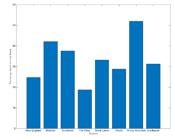
Figure 2 shows the share of loans made by small banks. In the states that make up the Rocky Mountain Region, on average, a little more than half of loans are made by small banks. While, in the Far West Region, this same percentage is less than 20%.
3.3. Real estate sector
The difference in the structure of the real estate market among states can also contribute to the heterogeneous behavior of agents in response to uncertainty shocks. According to Mumtaz (2018), for example, a high vacancy rate can signal the inability or reluctance of agents to absorb negative shocks. Furthermore, as Thanh et al. (2020) show, uncertainty shocks negatively affect the real estate market, so differences in this market across states can lead to different impacts among them.
Figure 3 presents the vacancy rate for rental properties, defined as the proportion of vacant properties among those available for rent. While the states that make up the Southeast Region have a higher vacancy rate, in the states in the Far West and Rocky Mountain regions this vacancy rate is lower. Therefore, in the first case, agents are more incapable or reluctant to absorb negative shocks, possibly leading to larger impacts.

3.4. Fiscal conditions
Finally, the intensity of uncertainty shocks can vary according to the government’s ability to support citizens in the face of a drop in income or job prospects (Mumtaz et al., 2018). On the one hand, if the uncertainty shock causes a drop in income, employment, and consumption, it may reduce government revenues leading to a drop in spending, which further accentuates the recession.9 On the other, states that spend more on welfare policies can offset the recessive effects, reducing the adverse impacts on employment and family income.
Figure 4 presents the averages by region of the debt volume to the states’ total expenses. This is an indicator of the fiscal capacity of states, with higher values associated with less capacity to respond to adverse shocks in the economy. Once again, the data show that the fiscal situation differs among states, which may contribute to heterogeneous responses across state economies to uncertainty shocks.

The following section presents the methodology used in this paper.
4. Methodology
The methodology is divided into three steps. The first consists of constructing a measure of uncertainty for the real estate market for each state in the United States, based on the Jurado et al. (2015) and Thanh et al. (2020) methodology. With this measure in hand, the second step is to analyze the impacts of state-level real estate uncertainty shocks on personal income per capita, employment and unemployment rate in each state, through impulse-response functions obtained from the estimation of a Bayesian PVAR model, using hierarchical priors, in which uncertainty shocks are identified by imposing sign restrictions (Arias et al., 2018). In the final step, we conduct a cross-sectional regression analysis between the accumulated response of state-level impulse-response functions over a 20-quarter horizon (which we consider as our measure of intensity), due to an uncertainty shock, and a set of state characteristics. This analysis will help us evaluate how those characteristics are associated with heterogeneity in responses (Carlino et al., 1999; Mumtaz et al., 2018).
4.1. Data
State-level Uncertainty. To calculate the measure of state-level uncertainty, which will be explained in section 4.2, we use six series of the real estate market, between the second quarter of 1995 and the last quarter of 2017: House price index10, New Private Housing Units Authorized by Building Permits (1 unit)11 and New Privately Owned Housing Units Authorized (1 unit, 2 units, 3 to 4 units, and 5 or more units).12 Data are seasonally adjusted and log differentiated. The first is already quarterly, while the others are monthly. We calculate the average every three months to obtain the quarterly format. This data was extracted from Federal Reserve Bank of Saint Louis (FRED).13
We use a set of 246 macroeconomic variables, between the second quarter of 1995 and the last quarter of 2017, to construct the factors with which we condition the volatility of forecast errors of the real estate sector variables. The series are classified into 14 groups: National Income and Product Accounts (NIPA); Industrial production; Employment and Unemployment; Housing; Inventories, Orders and Sales; Prices; Profit and Productivity; Interest rate; Money and Credit; Family Balance Sheets; Exchange rates; Stock market; and Non-Family Balance Sheets. The data are in level, and among them, some are stationary in level, while others need to be transformed through differentiation or log differentiation to be considered stationary. The base was also extracted from FRED.14
PVAR Model. To perform the Bayesian PVAR, we use personal income per capita15, employment16, the unemployment rate and the real estate uncertainty measure constructed in the first step.17 The data are at the state level, seasonally adjusted, and cover the period between the second quarter of 1995 and the last quarter of 2017. The first was already on a quarterly basis, but the second and third were on a monthly basis, so we calculated the average every three months to obtain the quarterly format. To obtain personal income per capita, we divide personal income by the state population.18 This data was also from FRED. We choose these variables, as we want to investigate the impacts of real estate uncertainty shocks on the economy as a whole, but in section 6 we perform an exercise analyzing the effect of this uncertainty shock on variables in the real estate market itself (Thanh et al., 2020).
Cross-Sectional Regression. To perform the cross-sectional regression, the regressors are divided into four groups: production structure, degree of financial friction, real estate sector, and state-level fiscal condition.19 For the first group, we use the share of the manufacturing, financial, agriculture, construction, mining and government sectors to the state’s nominal GDP.20 To represent the second group, we use the share of loans from small banks21 and the share of small firms in terms of employment.22 To represent the structure of real estate markets, we use the proportion of properties occupied by the owners. Finally, the group that portrays the fiscal situation of each state is represented by the share of welfare expenses for each state.23
4.2. Measure of uncertainty for the real estate market
Following recent literature, we construct a measure of state-level real estate uncertainty by calculating the conditional volatility in the forecast error in the variables of this market (Jurado et al., 2015; Ludvigson et al., 2015; Thanh et al., 2020). The first step is to define which variables to condition the predictions on. The idea is to condition on a very large set of macroeconomic variables, possibly capturing all those present in the agents’ information set when they formulate their forecasts (Jurado et al., 2015).
However, this means facing a very large dimensionality problem, given the number of variables. In this sense, the literature has used the principal components method (Thanh et al., 2020).24 This technique allows estimating factors, I t , from a set of 246 macroeconomic time series, X t = (X 1t , ..., X 246t )′ , such that they represent the most important part of the data. We assume that X t has a factor structure approximated as follows:
where is a vector of common latent factors, is the vector of correlation coefficients between the observed variables and the common latent factors and is a vector of idiosyncratic errors.
The second step is to calculate the expected values of the six real estate market variables in each state, , conditioned on the factors we estimated in the previous step, , resulting in , which is the forecast component of the series. The subscript represents the real estate market variables and represents the states. Predictions of housing variables for periods can be obtained through a diffusion index prediction model, that is, an augmented factor prediction model:
where and are polynomials of finite order in the lag operator of orders and , respectively. After that, the prediction error of these variables is calculated one step ahead and then recursively for longer horizons (Thanh et al., 2020).
The third step is to estimate the conditional volatility of these forecast errors to the factors, using a parametric stochastic volatility model. It generates six real estate market uncertainty indicators for each state, :
Finally, the State Real Estate Uncertainty (SREU) measure is a weighted average of these six indicators:
where and . Figures 20 and 21, in the appendix, present the estimates for the SREU for each state. The objective of constructing this indicator is, in addition to the indicator itself, to evaluate the impacts of a sectorial shock on the state’s economic dynamics on personal income per capita, the level of employment and the unemployment rate. For this, we obtain impulse response functions from a hierarchical Bayesian PVAR, which will be presented below.
4.3. Bayesian panel VAR
To analyze the impact of real estate uncertainty shocks on state-level real economic activity, we use a Bayesian panel VAR (PVAR) model with hierarchical priors, represented by:
where, α i and τ t are the state and time fixed effects, τ it is a linear time trend specific to state i, Y it is the measure of real activity (real income, employment, and unemployment rate) for each state i, P is the number of lags, and SREU it is the measure of uncertainty of the real estate market in state i, which varies over time. In the model, this measure is endogenous and evolves as follows:
where denotes the set of instruments uncorrelated with and:
A hierarchical prior will be used for the regression coefficients
where indicates the cross-sectional weighted average of the coefficients and is a diagonal matrix with diagonal elements, reflecting the scale of the individual elements of . The degree of pooling is determined by the parameter When , the coefficients become homogeneous between states. On the other hand, larger values of imply heterogeneous effects. is considered unknown and its posterior distribution is approximated by the estimation algorithm. This allows us to estimate the impact of uncertainty for the mean state while allowing for heterogeneity. The prior for the variance that controls the degree of pooling of the model, , has an Inverse Gamma distribution with parameters . We follow the recommendation of Jarocinski (2010), who says that this prior can be problematic, as the results are very sensitive to the choices of and . Because of this, he suggests that their values should be small. Thus, we choose and .
Regarding the parameters that represent a measure of specific variation between variables, a scaling coefficient that controls the speed of convergence of coefficients with lags greater than one, and a variance parameter for exogenous variables, we follow Dieppe et al. (2016) and set them to 0.5, 1 and 100, respectively. We run a total of 50,000 iterations, discarding the first 25,000. For the posterior estimation, we use the Gibbs sampling algorithm to obtain the draws. Identification strategy. We use signal restrictions on the Impulse Response Functions (IRF) to identify the real estate uncertainty shock. The restrictions are only imposed on the contemporary impact (Arias et al., 2018). The restrictions assume that, after a shock that increases the real estate uncertainty, personal income per capita and employment fall as a result, and the unemployment rate increases. The underlying idea is that, at least at impact, an increase in uncertainty has recessive effects (Bloom, 2009; Ludvigson et al., 2015; Leduc and Liu, 2016; Mumtaz et al., 2018). Table 1 presents the expected signs of the IRFs of the variables in the PVAR model in response to a real estate uncertainty shock.
The analysis of IRFs in response to a real estate uncertainty shock allows us to evaluate not only how each state responds to this shock but also whether there is heterogeneity in the responses among them. If this occurs, the next step is to understand which state-level characteristics can help explain this heterogeneity. The next section explains the strategy for this step.
4.4. Cross-sectional regression
Once the impact of real estate market uncertainty on real activity has been analyzed, we can investigate possible reasons for the differences in responses across states (Carlino et al., 1999; Mumtaz, 2018; Mumtaz et al., 2018). To do this, we estimate a cross-sectional regression model as follows:
where denotes the accumulated result of the impulse-response function, over a horizon of h = 20 quarters of the personal income per capita, employment and unemployment rate of the state , faced with a shock of uncertainty. β 0 is the intercept, R j refers to regional dummies, defined by the U.S. Bureau of Economic Analysis and the X i represent proxies that attempt to capture the role of different state-level characteristics in their responses to an uncertainty shock. We selected regressors that represent the sectorial structure of the states, the degree of financial friction, the structure of the housing market, and finally, the fiscal condition of each state.
5. Results
5.1. Uncertainty measure of the real estate market
In this section, we present the results of the state-level uncertainty measure of the real estate market. Figure 5 presents the median of SREU between the second quarter of 1995 and the last quarter of 2017. As Bloom (2009), Jurado et al. (2015) and Thanh et al. (2020), we include a dashed horizontal line that indicates 1.65 standard deviations above the uncertainty series mean to represent periods of high uncertainty. The SREU measure reached its peak at the time of the 2008-2009 Great Recession, which is consistent with the fact that the crisis originated in the real estate sector (Gertler and Gilchrist, 2018).

Figure 6 presents the medians of SREU throughout the period for each state. Using this indicator, state-level results point to higher levels of uncertainty, throughout the period, in New Mexico (11.28), Maryland (11.11), and New Jersey (8.21). While Idaho (0.67), Minnesota (0.75), and Maine (0.76) show smaller magnitudes.

Our results point to heterogeneity in levels of real estate uncertainty across states, with some having higher levels of uncertainty than others. Next, we assess whether state-level real estate uncertainty shocks affect the economies. Then, we investigate whether there is evidence of heterogeneous responses and, finally, which state-level characteristics can explain the heterogeneity in the impacts of uncertainty.25 In section 6, we will compare the SREU with other alternative measures of uncertainty.
5.2. Impulse-response functions to one standard deviation shock in State Real Estate Uncertainty - SREU
As discussed in Section 4.3, the evaluation of the effects of shocks to state-level real estate market uncertainty on real activity is conducted through the analysis of impulse response functions obtained from estimating a Bayesian Panel Vector Autoregressive (PVAR) model with hierarchical prior and identification through sign restrictions.
Our results indicate that following a shock that increases state-level real estate uncertainty, personal income per capita and employment decrease, while the unemployment rate rises across all states.26 Figure 7 displays the median state-level results of the impulse response functions for personal income per capita, employment, and the unemployment rate in response to a one standard deviation shock in the measure of state-level real estate uncertainty.

Impulse-response functions to one standard deviation shock in State Real Estate Uncertainty - SREU
Note: Impulse-Response Functions to one-standard deviation shock in state-level real estate uncertainty. The solid line represents the median of state responses to a state-level real estate uncertainty shock. The dashed lines represent the 68% credibility interval. Responses are multiplied by 100 to depict the percentage variation. Source: Authors’ elaboration.
In quantitative terms, a shock of one standard deviation shock in state-level real estate uncertainty leads to a decrease of approximately 0.2% in personal income per capita, a decrease of nearly 0.07% in employment, and an increase of around 0.7% in the unemployment rate. By the eighth quarter, the uncertainty effect reaches its peak, with respective values of -0.35%, -0.24%, and 1.89%, gradually dissipating only by the twentieth quarter, indicating a long-lasting shock.
These results reveal that a sectorial uncertainty shock can impact the aggregate economy, and its effects are typically recessionary. These recessionary impacts support the findings in the literature that empirically assess the impacts of macroeconomic uncertainty shocks (aggregate shocks) on economies (Bloom, 2009; Bachmann et al., 2013; Jurado et al., 2015; Baker et al., 2016; Mumtaz, 2018; Mumtaz et al., 2018). They also show that developments in the real estate sector have repercussions that spill over into the aggregate economy. Iacoviello (2005) and Iacoviello and Neri (2010) emphasize the importance of the real estate sector for real economic activity in the United States. The fact that real estate is used as collateral for loans can be one of the transmission channels between shocks in this sector and the effects on the rest of the economy. Relating this to uncertainty, through the real options channel, elucidated by Bernanke (1983), we can explain the countercyclical effect of real estate market uncertainty on the real economic activity in the United States.
According to this channel, an environment of high uncertainty creates a sense of unpredictability and financial instability about the future. Consequently, purchasing property becomes a risky decision as it cannot be undone easily, and reversing it would incur significant costs. Therefore, agents tend to reduce their real estate consumption when faced with an uncertainty shock.
According to the law of demand and assuming price flexibility, with fewer people buying properties, their prices fall. As the value of properties serves as collateral for loans, a lower loan value would be obtained. With this reduction, people would lower consumption of other goods. In response to this, firms would reduce the number of employees and the wages of those who remain employed, aiming to reduce their costs. This would lead to a reduction in personal income and an increase in the unemployment rate (Iacoviello and Neri, 2010; Christou et al., 2017).
Analyzing the state-level responses and using the accumulated responses over 20 periods, IRF 20 for each state, as a synthetic indicator, it is possible to observe that the responses of personal per capita income, employment, and unemployment rate to a state-level real estate uncertainty shock are heterogeneous across states. Although qualitatively the responses are similar, with a decline in income and employment, and an increase in the unemployment rate in all states, in some states, the impacts of the shocks are more pronounced.
Regarding personal per capita income, for example, the states of Louisiana (-11.69), North Dakota (-10.01), and Wyoming (-9.88) experienced a more pronounced decline, while Pennsylvania (-3.88), Maryland (-4.18), and Kentucky (-4.38) exhibited a smaller magnitude. Figure 8 presents the state-level results for personal per capita income.

Responses of personal income per capita to one standard deviation shock in State Real Estate Uncertainty - SREU
In terms of employment levels, Louisiana (-10.17), Wyoming (-5.89), and North Dakota (- 5.89) experienced a larger decline, while Massachusetts (-2.41), New Jersey (-2.63), and Pennsylvania (-2.7) had a smaller impact. Figure 9 illustrates the state-wise results.
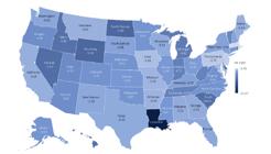
Employment Responses to one standard deviation shock in State Real Estate Uncertainty - SREU
Finally, regarding the unemployment rate, Louisiana (83.73), Wyoming (47.36), and Rhode Island (39.64) experienced a larger increase, while New Jersey (15.65), Massachusetts (16.12), and Arkansas (16.13) had a smaller increase. Figure 10 shows the state-level results.
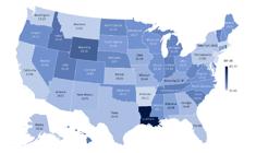
Responses of the unemployment rate to one standard deviation shock in State Real Estate Uncertainty - SREU
In sum, we observe heterogeneity in the responses of the state-level variables to real estate uncertainty shocks. Therefore, it is essential to investigate the factors associated with these differences. Possible explanations for these heterogeneities will be explored in the next section.
5.3. Understanding the heterogeneity in state-level responses to a real estate uncertainty shock
To comprehend why states exhibit varying magnitudes in their responses to uncertainty shocks, we conduct a cross-sectional regression analysis. This analysis involves examining the relationship between a measure of intensity of impacts and a set of variables that represents the production structure, the degree of financial friction, the real estate market, and the fiscal stance across states. We use the cumulative impulse-responses of personal income per capita, employment, and unemployment rate over a 20-quarter horizon as a measure of intensity.27
Table 2 presents the results of this cross-sectional regression. Columns (1) to (4) display the cumulative impulse-response functions of personal income per capita as dependent variables, with variations introduced by the inclusion of a set of variables that represents state heterogeneities. Columns (5) and (6) show the cumulative impulse-response functions of employment and unemployment rate as dependent variables, linking them to variables representing state-level economic sectors, the degree of financial friction, state fiscal conditions, and the structure of the real estate sector.
In column (1), when only the group representing the production structure is included in the set of regressors, only the one representing the public sector’s share in the state GDP shows a statistically significant coefficient. The negative coefficient indicates that states with a higher share in the GDP of this sector suffer larger negative impacts from uncertainty shocks on personal income per capita. Possibly, an uncertainty shock, as shown in the previous section causes a decline in income and employment, which may result in a decrease in revenue, reducing the state’s capacity to offset the adverse effects of uncertainty shocks.
In column (2), when the variables representing the degree of financial friction are included, the results show that the higher the share of manufacturing, the greater the adverse impacts of uncertainty shocks. Fasani and Rossi (2018) show that an uncertainty shock can lead to an increase in inflation, and in response the central bank may raise interest rates, accentuating the decline in output and consumption. Carlino et al. (1999) point out that the manufacturing industry is more sensitive to interest rate hikes, so when an uncertainty shock raises inflation and interest rates, states with a higher share of manufacturing end up experiencing a greater income decline. The results also show that the higher the share of the construction sector in the GDP, the greater the decline in personal income per capita in response to a real estate market uncertainty shock. As indicated earlier, uncertainty shocks negatively affect this sector with declines in property prices, construction employment, and new constructions (Thanh et al., 2020). As we will in subsection 6.3, the state-level real estate uncertainty shock has similar effects on employment in the construction sector and property prices, with persistent declines.
The negative coefficient associated with the financial sector’s proportion of GDP reinforces the idea that the impact of a real estate uncertainty shock on income per capita is larger in states with a higher share of this sector in the economy. Popp and Zhang (2016) show that uncertainty shocks have adverse effects on the real economy and financial markets. Moreover, they show that the effects are greater during recessions and reveal the importance of the financial channel in transmitting uncertainty shocks.
In column (3), when the variable representing the responsiveness of the states is added, the results show that the higher the share of small banks in total loans, the greater the impact of uncertainty shocks. As indicated in section 3, this variable represents the degree of financial friction of firms and households (Carlino et al., 1999). According to Kashyap and Stein (1995), the size of banks affects their ability to finance loans, which, in the face of a recessionary shock, ends up accentuating the adverse effects on income per capita, in a mechanism similar to the financial accelerator of Bernanke et al. (1999). The results also indicate that the higher the states’ spending on welfare policies, the lesser the adverse impacts of uncertainty shocks. This suggests that the greater the state’s ability to offer a social safety net to families, in a recessionary scenario, the smaller the decline in family income.
The column (4) adds to the previous one the variable representing the heterogeneity of the real estate market structure. Compared to the results of column (3), the results remain unchanged, although there is a decrease in the magnitude of the coefficients. However, the results reveal that the structure of the real estate market seems not to matter for the heterogeneity of the per capita income response to uncertainty shocks.
Column (5) uses the cumulative employment responses as the dependent variable and regressors representing the four groups of variables. In the employment response, the coefficients of the public sector and welfare policy spending were significant. A similar explanation to that used in the case of per capita income can be given for employment. If an uncertainty shock causes a decrease in revenue, it may reduce the state’s ability to offset the adverse effects of uncertainty, and therefore, greater impacts on employment (and income) are expected. On the other hand, states that spend more on welfare policies can offset the adverse effects on employment. The positive coefficient associated with this variable suggests that this is the case. A counterintuitive result is the positive and statistically significant coefficient of the variable representing small firms. This means that the impacts on employment are smaller in states with a higher proportion of employment in firms with up to 250 employees.
Finally, column (6) uses the cumulative responses of the unemployment rate as the dependent variable and regressors representing the four groups of variables. In this case, states with a higher share of agriculture experience higher increases in the unemployment rate. Sun et al. (2021) show that uncertainty shocks can negatively affect agricultural commodity prices, and therefore, states, where the agricultural sector has a higher share of GDP, may experience greater increases in the unemployment rate. The coefficients associated with manufacturing and financial sector participation are also positive, indicating similarly that states where these sectors have a greater presence in GDP experience higher increases in the unemployment rate. The transmission mechanisms are the same as already discussed in the case of per capita income.
6. Additional results
This section presents some additional analysis using our uncertainty measure. Initially, subsection 6.1 compares the state-level real estate uncertainty measure with two national uncertainty measures. Next, subsection 6.2 presents a comparison of IRFs in response to a national real estate uncertainty shock, using the measure constructed by Thanh et al. (2020), and our state- level measure. Subsection 6.3 shows the IRFs in response to a shock of real estate uncertainty in real estate market variables. Finally, subsection 6.4 evaluates the robustness of the results by presenting the IRFs in response to a real estate uncertainty shock using a recursive identification scheme.
6.1. State-level real estate uncertainty measure and aggregate measures
Figure 11 presents a comparison of our State Real Estate Uncertainty measure (SREU), with the national real estate uncertainty measure created by Thanh et al. (2020), which we label as National Real Estate Uncertainty (NREU) and the measure of macroeconomic uncertainty, created by Jurado et al. (2015), referred to as National Macroeconomic Uncertainty - NMU. We include a dashed horizontal line indicating 1.65 standard deviations above the mean of each series to represent periods of high uncertainty. All series range from the second quarter of 1995 to the second quarter of 2017.
All uncertainty measures presented a high level during the 2008-2009 crisis period, of which the SREU presents the highest peak. It is also observed that after this period, the NMU drops considerably, while the NREU remains high, falling slightly, but without returning to the original level. SREU also falls, but at a slower rate than NMU, ending the series at a higher level than at the beginning of it. This observation corroborates the results of Thanh et al. (2020), which note that uncertainty in the real estate market lasted considerably longer than general economic uncertainty.
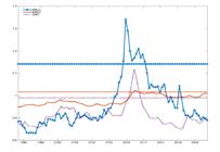
Table 3 presents the mean and standard deviation of the SREU, NREU, and NMU measures. They have similar means, but the SREU has a higher standard deviation, probably because it represents the median of the uncertainty across 51 states.
6.2. Impulse Responses to Different Uncertainty Measures
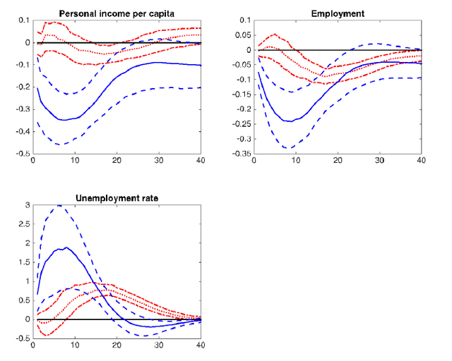
Figure 12 depicts the median results of state-level impulse response functions for personal income per capita, employment, and the unemployment rate following a shock of one standard deviation in SREU, as previously shown in Figure 7, and a shock of one standard deviation in the measure of national real estate uncertainty (NREU) constructed by Thanh et al. (2020).28

The impulse response functions for the three variables are qualitatively similar and significant for both uncertainty measures. By construction, personal income per capita and employment exhibit a negative response to a positive uncertainty shock at impact, while the unemployment rate responds positively. These findings are in line with Mumtaz (2018), Mumtaz et al. (2018), and Jurado et al. (2015). Possible explanations for these behaviors are discussed in Section 5.2.
6.3. Impulse-Response Functions of Real Estate Variables
We also analyze the impact of our state-level uncertainty measure on some variables of the real estate sector. To achieve this, we redefine our uncertainty measure, excluding the real estate price index to enable its utilization in the Bayesian Panel Vector Autoregression (PVAR). Subsequently, we estimate the Bayesian PVAR with a hierarchical prior, identification through sign restrictions with four lags.
The variables included in the PVAR model are personal income per capita, (total) employment, and (total) unemployment rate, which are the same variables used in the PVAR of Section 5.2.29 Additionally, we include the real estate price index mentioned in Section 4.1 and employment in the construction sector.30 As we were unable to find a specific employment variable for the real estate construction sector at the state level, we used state-level employment in the construction sector to represent it, as the housing sector is encompassed within it.
The expected signs of the first three variables have been presented in Table 1. As for the last two variables, an increase in uncertainty in the real estate market is expected to result in a reduction in real estate prices and a decrease in employment levels in the construction sector. These expected signs follow Thanh et al. (2020), which find that a positive shock (increase) in real estate uncertainty leads to a reduction in real estate prices and employment in the construction sector.
Figure 13 presents the median state-level results of the impulse-response functions of personal income per capita, total employment, total unemployment rate, employment in the construction sector, and real estate prices in response to a one standard deviation shock in state-level real estate uncertainty. It is observed that, by construction and with significance, in the impact period, personal income per capita, total employment, employment in the construction sector, and real estate prices respond negatively to a positive uncertainty shock, while the unemployment rate rises. These effects persist beyond the impact period (sign restriction period) and are significant.

The explanation for this behavior complements what was discussed in Section 5.2. Through the real options channel and the irreversibility character of real estate purchases, when facing a real estate market uncertainty shock, individuals would choose to reduce their real estate consumption.
By the law of demand and assuming flexibility in prices and the possibility of using real estate as collateral for loans, with fewer people buying real estate, prices would fall, and a lower loan value would be obtained. With this reduction, people would consume even less of other goods as well. In response to this, firms would reduce hiring in this sector and decrease the wages of employees who remain employed, aiming to reduce their costs, which would decrease income and increase the unemployment rate accordingly. Given the significance of this sector in the United States economy and its integration into other sectors, there is a chain effect, negatively affecting employment and income.
Furthermore, we add the impact of these variables due to one standard deviation in our state- level real estate uncertainty (baseline). The impulse response functions for the five variables are qualitatively similar and significant for both uncertainty measures.
6.4. Impulse-Responses Functions with Recursive Identification
Finally, we use a recursive identification scheme to obtain the real estate uncertainty shock. We follow Mumtaz (2018) and ordered the variables as follows: a measure of real estate uncertainty, personal income per capita, employment, and unemployment rate. Figure 14 displays the median of the state-level results of the impulse-response functions for personal income per capita, employment, and the unemployment rate following a one standard deviation shock in SREU. The results exhibit qualitative similarity.

Impulse-Response Functions to State-level Real Estate Uncertainty Shock - Recursive Identification
7. Final remarks
In this paper, we investigate the effects of a shock of uncertainty originating from the real estate sector on real activity across states in the US. To do this, we construct a measure of state-level real estate uncertainty and use this measure in a Bayesian hierarchical PVAR model. We use sign restrictions to identify the state-level real estate uncertainty shock. Finally, we implement a cross-sectional regression to investigate possible explanations for state-level heterogeneities in responses to real estate uncertainty shocks.
Our results indicate high levels of uncertainty in all states during the 2008-2009 financial crisis but with different magnitudes and dynamics among them. Second, they reveal that a real estate uncertainty shock has adverse impacts on personal income per capita, employment, and the unemployment rate in all states, but with heterogeneous effects. As highlighted, these results reveal that developments in the real estate sector have spillover effects on the economy and can help explain state-level recessions and expansions. The results also show adverse effects on property prices and employment in the construction sector.
The cross-sectional regression results show that states with a higher share of GDP in the financial sector, construction, and manufacturing industry, and with a higher degree of financial friction tend to be more adversely affected by uncertainty shocks. Conversely, states with higher spending on social welfare policies tend to be less affected.
Therefore, these results reveal that heterogeneity in economic sectors influences state-level responses to real estate uncertainty shocks. Additionally, they allow for an expanded understanding of new sources of uncertainty that can explain state-level expansions and recessions, not necessarily related to aggregate variables. Finally, they may help policymakers in designing compensatory policies in response to crises originating in the real estate sector.
ACKNOWLEDGMENTS
We thank Andreza Palma, Igor Ézio, Paulo Vaz, Rafael Vasconcelos, Roberto Perrelli, and two anony mous referees for their comments. We also thank participants at the 50º Encontro Nacional de Economia(ANPEC). The usual disclaimer applies. Marcelo thanks CNPq for financial support under the grant 421701/2016-1.João Pedro M. Silva provided excellent research assistance.
References
- Alessandri, P. and H. Mumtaz (2019). Financial regimes and uncertainty shocks. Journal of Monetary Economics 101, 31-46.
- Arias, J. E., J. F. Rubio-Ramírez, and D. F. Waggoner (2018, March). Inference Based on SVARs Identified with Sign and Zero Restrictions: Theory and Applications. Econometrica 86(2), 685-720.
- Bachmann, R., S. Elstner, and E. R. Sims (2013). Uncertainty and economic activity: Evidence from business survey data. American Economic Journal: Macroeconomics 5(2), 217-49.
- Baker, S. R., N. Bloom, and S. J. Davis (2016). Measuring economic policy uncertainty. The quarterly journal of economics 131(4), 1593-1636.
- Bernanke, B. S. (1983). Irreversibility, uncertainty, and cyclical investment. The quarterly journal of economics 98(1), 85-106.
- Bernanke, B. S., M. Gertler, and S. Gilchrist (1999). The financial accelerator in a quantitative business cycle framework. Handbook of macroeconomics 1, 1341-1393.
- Bloom, N. (2009). The impact of uncertainty shocks. Econometrica 77(3), 623-685.
- Carlino, G. and R. DeFina (1998). The differential regional effects of monetary policy. Review of economics and statistics 80(4), 572-587.
- Carlino, G., R. DeFina, et al. (1999). Do states respond differently to changes in monetary policy. Business Review 2, 17-27.
- Christou, C., J. Cunado, R. Gupta, and C. Hassapis (2017). Economic policy uncertainty and stock market returns in pacific-rim countries: Evidence based on a bayesian panel var model. Journal of Multinational Financial Management 40, 92-102.
- Dieppe, A., B. van Roye, and R. Legrand (2016, July). The BEAR toolbox. Working Paper Series 1934, European Central Bank.
- Dunteman, G. H. (1989). Principal components analysis. Number 69. Sage.
- Fasani, S. and L. Rossi (2018). Are uncertainty shocks aggregate demand shocks? Economics Letters 167, 142-146.
- Gertler, M. and S. Gilchrist (2018). What happened: Financial factors in the great recession. Journal of Economic Perspectives 32(3), 3-30.
- Husted, L., J. Rogers, and B. Sun (2020). Monetary policy uncertainty. Journal of Monetary Economics 115, 20-36.
- Iacoviello, M. (2005). House prices, borrowing constraints, and monetary policy in the business cycle. American economic review 95(3), 739-764.
- Iacoviello, M. and S. Neri (2010). Housing market spillovers: Evidence from an estimated DSGE model. American Economic Journal: Macroeconomics 2, 125-164.
- Jarocinski, M. (2010). Responses to monetary policy shocks in the east and the west of Europe: a comparison. Journal of Applied Econometrics 25(5), 833-868.
- Jurado, K., S. C. Ludvigson, and S. Ng (2015). Measuring uncertainty. American Economic Review 105(3), 1177-1216.
- Kashyap, A. K. and J. C. Stein (1995). The impact of monetary policy on bank balance sheets. In Carnegie-Rochester conference series on public policy, Volume 42, pp. 151-195. Elsevier.
- Leduc, S. and Z. Liu (2016). Uncertainty shocks are aggregate demand shocks. Journal of Monetary Economics 82, 20-35.
- Ludvigson, S. C., S. Ma, and S. Ng (2015). Uncertainty and business cycles: exogenous impulse or endogenous response? Technical report, National Bureau of Economic Research.
- McCracken, M. and S. Ng (2020). Fred-qd: A quarterly database for macroeconomic research. Technical report, National Bureau of Economic Research.
- Mumtaz, H. (2018). Does uncertainty affect real activity? evidence from state-level data. Eco- nomics Letters 167, 127-130.
- Mumtaz, H., L. Sunder-Plassmann, and A. Theophilopoulou (2018). The state level impact of uncertainty shocks. Journal of Money, Credit and Banking 50, 1879-1899.
- Ng, E. C. (2015). Housing market dynamics in China: Findings from an estimated DSGE model. Journal of Housing Economics 29, 26-40.
- Popp, A. and F. Zhang (2016). The macroeconomic effects of uncertainty shocks: The role of the financial channel. Journal of Economic Dynamics and Control 69, 319-349.
- Sun, T.-T., C.-W. Su, N. Mirza, and M. Umar (2021). How does trade policy uncertainty affect agriculture commodity prices? Pacific-Basin Finance Journal 66, 101514.
- Thanh, B. N., J. Strobel, and G. Lee (2020). A new measure of real estate uncertainty shocks. Real Estate Economics 48(3), 744-771.
-
1
Carlino and DeFina (1998) and Carlino et al. (1999) provide evidence of differentiated effects of monetary policy shocks in different U.S. regions and states, respectively. More related to our work, Mumtaz et al. (2018) show evidence that macroeconomic uncertainty shocks have differentiated effects on states, and differences in the economic structure of states help explain such heterogeneous effects.
-
2
For space reasons, measures of real estate uncertainty for each state are presented in the online appendix.
-
3
For space reasons, the IRFs for each state in response to an uncertainty shock are presented in the online appendix.
-
4
According to Jurado et al. (2015), the idea of eliminating the predictable component of the series when constructing the measures is that, for them, uncertainty is associated with the loss of the forecasting ability of variables.
-
5
States differ substantially in terms of their share in the GDP of the manufacturing, the financial sector, and the degree of financial friction (Carlino et al., 1999). Associating these state diversities with their responses to uncertainty shocks is important to investigate the transmission channels through which these shocks affect state economies.
-
6
They searched, in articles in the 10 main newspapers in the United States since 1985, for combinations of words between the following three groups: Economic or economy; uncertain or uncertainty and one or more of congress, deficit, Central Bank, legislation, regulation or White House.
-
7
The authors define a large uncertainty when it exceeds 1.65 standard deviations above its mean.
-
8
Our results also point to declines in property prices and construction employment in states following a state-level real estate uncertainty shock.
-
9
According to the Tax Policy Center, on average, 42% of state revenues came from sales and income taxes in 2017. Only 1/3 came from intergovernmental transfers. Source: https://www.taxpolicycenter.org/ briefing-book/what-are-sources-revenue-state-governments. Accessed on 12/15/23.
-
10
The original name of the series is All-Transactions House Price Index and is estimated using housing sale prices.
-
11
This series represents the total number of building permits for structures with 1 unit, that is, with one property, which is built with public subsidy, partially or fully.
-
12
This series represents the total number of building permits for structures that are not built with public subsidy and are not owned by the government. The unit quantity, for example, 1 unit, 2 units, 3 to 4 units, or 5 or more units, refers to the quantity of properties per structure.
-
13
Thanh et al. (2020) uses forty real estate market series, but of these, only six have information at the state level.
-
14
For more details see McCracken and Ng (2020).
-
15
Personal income is the income that people receive in exchange for their supply of labor, land and capital used in current production and the net current transfer payments they receive from companies and the government. personal income per capita is personal income divided by the state’s population.
-
16
This employment measure is all employees total nonfarm and represents the number of workers that excludes owners, private domestic employees, unpaid volunteers, agricultural employees, and unincorporated self-employed people, that is, not constituted in a legal society. This measure constitutes 80% of the workers contributing to the United States GDP.
-
17
The employment and unemployment rate variables were included to represent the dynamics of the job market (Mumtaz et al., 2018). Although related, they can move differently in response to uncertainty shocks. For example, assuming that in response to an uncertainty shock, there is lower participation in the labor market, with a drop in the economically active population and proportional drops in employment and unemployment. In this case, although the level of employment falls, the unemployment rate would remain constant. On the other hand, if the response is an increase in the labor supply, in response to an adverse shock, the employment level may remain constant, but the unemployment rate will rise.
-
18
The state population is only reported annually, so as Mumtaz et al. (2018) a linear interpolation was implemented to obtain the quarterly format and thus use it to construct personal income per capita.
-
19
We thank Haroom Mumtaz for kindly providing the data for this stage.
-
20
These data were taken from the U.S. Bureau of Economic Analysis and are an average between annual data from 1963 to 2013.
-
21
This data was taken from Call Reports, FFIEC and they are an average between the first quarter of 2001 and the third quarter of 2015.
-
22
These data are from the Census Bureau, County Business Patterns and are an annual average from 1986 to 2013.
-
23
According to the Urban Institute, these expenses include cash assistance through Temporary Assistance for Needy Families (TANF), Supplemental Security Income, and other payments made directly to individuals, as well as payments to doctors and other service providers under programs such as Medicaid.
-
24
This is a statistical technique that linearly transforms an original set of variables into a substantially smaller set of uncorrelated variables, which represent most of the information in the original set. Its objective is to reduce the dimensionality of the original data set (Dunteman, 1989).
-
25
For reasons of space, the figures of state-level uncertainty measures are in the online appendix.
-
26
Due to space constraints, state-level IRFs are presented in Figures 15 to 19 in the online Appendix.
-
27
We decide to use this measure because after the 20th quarter, we cannot reject the hypothesis that the IRFs are null.
-
28
The Bayesian method allows to estimate the PVAR model with sign restrictions on the IRFs using national and state-level variables. We impose the same sign restrictions on the IRFs to obtain the one standard deviation shock to NREU.
-
29
In Section 5.2, these variables are denoted as employment and unemployment rate, but to differentiate from construction employment, in this section, they are denoted as total employment and total unemployment rate.
-
30
The original name of this employment measure is all employees, construction, and according to FRED, it represents construction employees in the construction sector, including Work supervisors, skilled craftsmen, mechanics, apprentices, helpers, workers, etc., in construction or in workshops or shipyards in tasks (such as pre-cutting and pre-assembly) usually performed by members of the construction professions.
A. Online appendix
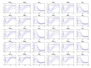
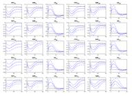
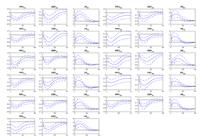
A.1. State-level impulse response functionsThe following figures present the state-level impulse response functions, obtained from the estimation of the hierarchical Bayesian PVAR where the identification of the uncertainty shock was carried out by imposing signal restrictions.


A.2. State Real Estate Uncertainty - SREU
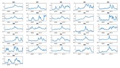
The following figures present measures of housing uncertainty for each state in the United States.

Edited by
-
EDITOR-CHEFE
Dante Mendes Aldrighi https://orcid.org/0000-0003-2285-5694 Professor - Department of Economics University of São Paulo (USP)

 Note: The figure shows the composition of GDP by economic sector. The data is the sectorial average among the states that make up each region. Source: Authors’ elaboration.
 Note: Small banks are defined as at or below the 90th percentile of the national distribution of bank size by assets. Source: Authors’ elaboration.
 Note: The vacancy rate for rental properties is defined as the proportion of vacant properties among those available for rent. Source: Authors’ elaboration.
 Note: The figure shows the regional average of state-level debt as a share of total expenditure. Source: Authors’ elaboration.
 Note: The solid line represents the median of state-level real estate uncertainties, SREU, between the second quarter of 1995 and the last quarter of 2017. The dashed horizontal line indicates 1.65 standard deviations above the series average, representing periods of high uncertainty. Source: Authors’ elaboration.
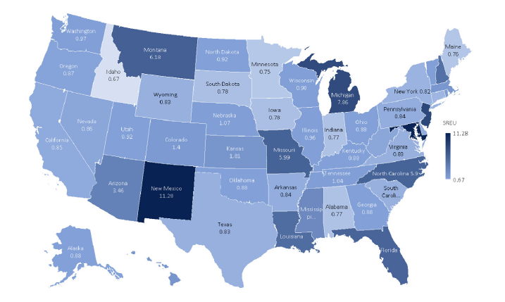 Note: The map shows the median, for each state, of the State Real Estate Uncertainty - SREU between the second quarter of 1995 and the last quarter of 2017. Darker colors reflect higher levels of uncertainty. Source: Authors’ elaboration.

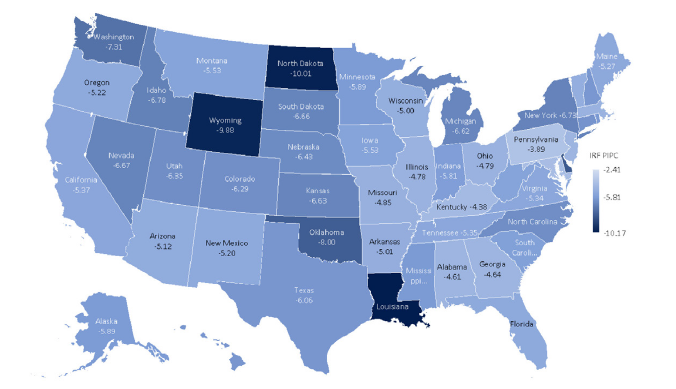 Note: The map depicts the cumulative responses of personal income per capita in each state to one standard deviation shock in state-level real estate uncertainty. Darker colors indicate more pronounced responses to the state-level real estate uncertainty shock. Source: Authors’ elaboration.
 Note: The map displays the accumulated employment responses in each state to one standard deviation shock in state-level real estate uncertainty. Darker colors indicate more pronounced responses to the state- level real estate uncertainty shock. Source: Authors’ elaboration.
 Note(s): The map shows the cumulative responses of the unemployment rate in each state to one standard deviation shock in state-level real estate uncertainty. Darker colors indicate more pronounced responses to the state-level real estate uncertainty shock. Source: Authors’ elaboration.
 Note: The crossed line represents the median state real estate uncertainty (SREU), while the solid line represents national real estate uncertainty (NREU), created by
  Note: Impulse response functions to a one standard deviation shock in the real estate market uncertainty measure. The solid line represents the median state-level responses to a state real estate uncertainty shock created by this study. The red dotted line represents the median state-level responses to a national real estate uncertainty shock created by
  Note(s): Impulse response functions to a one standard deviation shock in the real estate market uncertainty measure. The solid line represents the median state-level responses to a state real estate uncertainty shock created by this study (baseline). The dotted line represents the median state-level responses to a national real estate uncertainty shock without a real estate price index. The dashed and dashed-dotted lines represent the 68% credibility interval. Responses are multiplied by 100 to depict the percentage variation. Source: Authors’ elaboration.
 Note(s): The solid blue line represents impulse response functions to a one standard deviation shock in the state-level real estate uncertainty with recursive identification. The solid red line represents the impulse response functions to a one standard deviation shock in the state-level real estate uncertainty with signal restriction identification (baseline). Dashed lines represent the 68% credibility interval. Responses are multiplied by 100 to depict the percentage variation. Source: Authors’ elaboration.
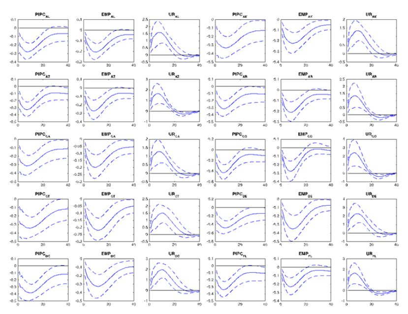 Note(s): Impulse-response functions to a one standard deviation shock in the real estate market uncertainty measure. The solid line represents the impulse-response functions of personal income per capita (PIPC), employment (EMP), and unemployment rate (UR) for Alabama (AL), Alaska (AK), Arizona (AZ), Arkansas (AR), California (CA), Colorado (CO), Connecticut (CT), Delaware (DE), District of Columbia (DC) and Florida (FL) to a one standard deviation uncertainty shock. The dashed lines represent the 68% credibility interval. Source: Authors’ elaboration.
 Note(s): Impulse-response functions to a one standard deviation shock in the real estate market uncertainty measure. The solid line represents the impulse-response functions of per capita personal income (PIPC), employment (EMP), and unemployment rate (UR) for Georgia (GA), Hawaii (HI), Idaho (ID), Illinois (IL), Indiana (IN), Iowa (IA), Kansas (KS), Kentucky (KY), Louisiana (LA) and Maine (ME) to a one standard deviation uncertainty shock. The dashed lines represent the 68% credibility interval. Source: Authors’ elaboration.
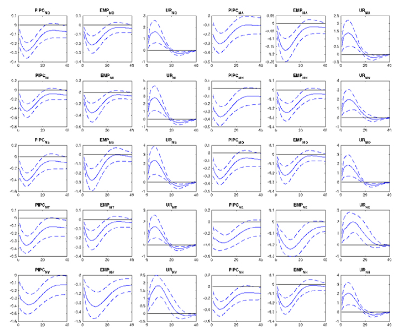 Note: Impulse-response functions to a one standard deviation shock in the real estate market uncertainty measure. The solid line represents the impulse-response functions of per capita personal income (PIPC), employment (EMP), and unemployment rate (UR) for Maryland (MD), Massachusetts (MA), Michigan (MI), Minnesota (MN), Mississippi (MS), Missouri (MO), Montana (MT), Nebraska (NE), Nevada (NV) and New Hampshire (NH) to a one standard deviation uncertainty shock. The dashed lines represent the 68% credibility interval. Source: Authors’ elaboration.
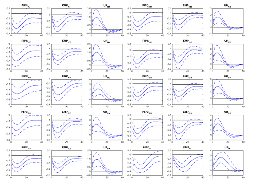 Note(s): Impulse-response functions to a one standard deviation shock in the real estate market uncertainty measure. The solid line represents the impulse-response functions of per capita personal income (PIPC), employment (EMP), and unemployment rate (UR) for New Jersey (NJ), New Mexico (NM), New York (NY), North Carolina (NC), North Dakota (ND), Ohio (OH), Oklahoma (OK), Oregon (OR), Pennsylvania (PA) and Rhode Island (RI) to a one standard deviation uncertainty shock. The dashed lines represent the 68% credibility interval. Source: Authors’ elaboration.
 Note(s): Impulse-response functions to a one standard deviation shock in the real estate market uncertainty measure. The solid line represents the impulse-response functions of per capita personal income (PIPC), employment (EMP), and unemployment rate (UR) for South Carolina (SC), South Dakota (SD), Tennessee (TN), Texas (TX), Utah (UT), Vermont (VT), Virginia (VA), Washington (WA), West Virginia (WV), Wisconsin (WI), and Wyoming (WY) to a one standard deviation uncertainty shock. The dashed lines represent the 68% credibility interval. Source: Authors’ elaboration.
 Note: State Real Estate Uncertainty - SREU in the states of Alabama (AL), Alaska (AK), Arizona (AZ), Arkansas (AR), California (CA), Colorado (CO), Connecticut (CT), Delaware (DE), District of Columbia (DC), Florida (FL), Georgia (GA), Hawaii (HI), Idaho (ID), Illinois (IL), Indiana (IN), Iowa (IA), Kansas (KS), Kentucky (KY), Louisiana (LA), Maine (ME), Maryland (MD), Massachusetts (MA), Michigan (MI), Minnesota (MN), and Mississippi (MS). Source: Authors’ elaboration.
 Note: State Real Estate Uncertainty - SREU in the states of Missouri (MO), Montana (MT), Nebraska (NE), Nevada (NV), New Hampshire (NH), New Jersey (NJ), New Mexico (NM), New York (NY), North Carolina (NC), North Dakota (ND), Ohio (OH), Oklahoma (OK), Oregon (OR), Pennsylvania (PA), Rhode Island (RI), South Carolina (SC), South Dakota (SD), Tennessee (TN), Texas (TX), Utah (UT), Vermont (VT), Virginia (VA), Washington (WA), West Virginia (WV), Wisconsin (WI), and Wyoming (WY). Source: Authors’ elaboration.