Crop water stress index of beans

ABSTRACT

A sustainable future requires efficient water use in irrigated agriculture to ensure food and water security. The crop water stress index (CWSI) is a remote sensing tool that can help achieve this goal. In typical CWSI experiments, infrared sensors focus on the canopy to measure its temperature. This study evaluated this methodology for crop beans (Phaseolus vulgaris L.) with low canopy coverage. In this scenario, the temperature measurement is significantly affected by the presence of straw mulch. The study also proposed a procedure that uses supplementary data to estimate canopy coverage and straw mulch temperature. Then, the canopy temperature is finally estimated from the infrared sensor measurement. The procedure was successfully implemented for low canopy coverages. Without it, the baseline slope was inconsistent with the CWSI theory. This was particularly true during the earlier phenological stages. The lowest observed canopy coverage was 0.17 for the baseline and 0.26 when estimating the CWSI. The CWSI showed a clear relationship with soil water content.

Key words
Phaseolus vulgaris L.; phenological stages; straw mulch; canopy temperature; canopy coverage

INTRODUCTION

Irrigated agriculture plays a crucial role in ensuring food and nutritional security. It improves yield and product supply, generates employment, and increases producer income. Irrigation also reduces production risks by mitigating the impacts of climate change. However, efficient water use is essential (Siyal et al. 2023).

Irrigated agriculture is fundamental to achieving the Sustainable Development Goals in the United Nations’ 2030 Agenda. This is particularly true for the agricultural sector. Among the United Nations’ goals, zero hunger and sustainable agriculture stand out (United Nations 2016). Food production requires a substantial volume of water, which must come from rainfall or irrigation.

Irrigation is also vital to the Brazilian agricultural economy. Brazil has 8.2 million hectares of irrigated land, ranking sixth globally in area. In contrast, this represents less than 1% of the Brazilian territory. Brazil has the potential for irrigation growth, unlike other leading countries in the ranking. The prospect by 2040 is a 76% increase in irrigated areas in Brazil (ANA 2021).

Nowadays, agriculture faces numerous challenges and opportunities. Thus, precision irrigation tools must be developed to promote water use efficiency. Remote sensing can enhance the monitoring of irrigated areas, improving spatial resolution and scale. In this context, the crop water stress index (CWSI) is an excellent alternative for assessing plant water status. CWSI normalizes the difference between canopy and air temperature. Its values range from 0 to 1, representing a plant’s well-watered status and severe water deficit, respectively.

The canopy temperature can be measured using handheld infrared thermometers (Idso et al. 1981), stationary infrared radiometer (IRR) sensors (Han et al. 2018, Gonzalez-Dugo et al. 2020), or thermal cameras (Katimbo et al. 2022, Sánchez-Piñero et al. 2022). CWSI correlates well with stem water potential and leaf conductance (Bellvert et al. 2016, Sánchez-Piñero et al. 2022). It has also been correlated with relative transpiration (Gonzalez-Dugo et al. 2020), leaf photosynthetic activity (Luan et al. 2021), crop yield (Gonzalez-Dugo et al. 2019), and soil water content (Katimbo et al. 2022).

Earlier studies on CWSI assessed crops such as squash, alfalfa, and soybeans (Idso et al. 1981), as well as sorghum, corn, beans, and cotton (O’Toole and Hatfield 1983). These studies measured only the canopy temperature and took precautions to avoid interference from the soil surface temperature. Since then, CWSI has been successfully applied to trees and other perennial crops, such as pistachio (Testi et al. 2008), persimmon (Ballester et al. 2013), citrus (Gonzalez-Dugo et al. 2014), peach (Bellvert et al. 2016), grapevine (Poblete-Echeverría et al. 2017), almond (Gonzalez-Dugo et al. 2020), and olive (Sánchez-Piñero et al. 2022). In those cases, measuring only the canopy temperature was more straightforward. Han et al. (2018) calculated the CWSI for maize. They adjusted the IRR sensor position several times during the plant cycle to ensure the canopy coverage was above 0.8.

This study used data from beans (Phaseolus vulgaris L.) planted with no-tillage and straw mulching. This technique promotes greater water retention in the soil surface and reduces the need for irrigation during the cultivation cycle (Cunha et al. 2015, Yin et al. 2023). This study evaluated the feasibility of obtaining the CWSI for canopy coverages below 0.8. It also proposed a procedure for estimating canopy coverage and straw mulch temperature. This study also correlated the CWSI with soil water content.

MATERIALS AND METHODS

The study was conducted in an experimental area in Campinas, São Paulo, Brazil. ‘Carioca’ beans (P. vulgaris L.) were planted in two cultivation cycles. The cultivar ‘IAC1850’ was planted in the first cycle, on August 7, 2023, and the cultivar ‘IAC2051’ in the second cycle, on February 6, 2024. The first cultivation cycle lasted 91 days, whereas the second lasted 82 days. Each cycle comprises five phenological stages: vegetative, development, flowering, grain-filling, and maturation.

Center-pivot irrigation was used on both cultivation cycles. Throughout the first cycle, the bean plants were kept well-watered. Twelve irrigations were carried out, totaling 131 mm of water; the recorded rainfall was 340 mm. In the second cycle, a severe water deficit occurred during flowering, while a mild one occurred during grain-filling and maturation. The total rainfall reached 256 mm, and 10 irrigations were performed, totaling 100 mm of water. The field capacity and the permanent wilting point were determined from the soil-water retention curve (Van Genuchten 1980).

The automatic meteorological station gathered data every 20 minutes. This station was located approximately 700 m from the experimental area. In addition to rainfall, it recorded air temperature, relative air humidity, solar radiation, and wind speed at 10 m above ground. Tables 1 and 2 show the average values of the meteorological data for each cycle. To estimate the net radiation every 20 minutes, a calculation tool (Mariano et al. 2011) provided daily net radiation values for each cycle. Then, the average ratio of net radiation to solar radiation was applied to the meteorological data.

Table 1
Meteorological data on the first cultivation cycle at each phenological stage. Average values: minimum and maximum air temperature, relative air humidity, solar radiation, and wind speed at 10 m above ground.

	Vegetative	Development	Flowering	Grain-filling	Maturation
Period (2023)	Aug 7 Aug 17	Aug 18 Sep 7	Sep 8 Sep 23	Sep 24 Oct 18	Oct 19 Nov 6
Days after planting	0–10	11–32	33–47	48–72	73–91
Maximum temperature (°C)	29.9	29.0	32.2	31.4	30.0
Minimum temperature (°C)	15.8	16.7	17.9	19.5	19.0
Maximum relative air humidity (%)	95.6	92.8	94.4	98.1	98.5
Minimum relative air humidity (%)	47.5	50.5	42.9	59.2	61.0
Solar radiation (MJ·m-2·day-1)	7.0	9.4	14.9	11.9	13.8
10 m wind speed (m·s-1)	0.4	1.3	2.2	2.8	2.7

Table 2
Meteorological data on the second cultivation cycle at each phenological stage. Average values: minimum and maximum air temperature, relative air humidity, solar radiation, and wind speed at 10 m above ground.

	Vegetative	Development	Flowering	Grain-filling	Maturation
Period (2024)	Feb 6 Feb 16	Feb 17 Mar 6	Mar 7 Mar 22	Mar 23 Apr 12	Apr 13 Apr 28
Days after planting	0–10	11–29	30–45	46–66	67–82
Maximum temperature (°C)	32.5	32.6	34.0	30.2	31.3
Minimum temperature (°C)	20.5	20.5	21.6	19.8	19.1
Maximum relative air humidity (%)	99.7	99.8	99.4	98.3	98.1
Minimum relative air humidity (%)	53.9	58.9	57.4	59.6	51.3
Solar radiation (MJ·m-2·day-1)	17.9	15.6	16.4	12.1	14.2
10 m wind speed (m·s-1)	1.7	1.7	1.7	2.0	2.2

Two SIL-411 IRR from Apogee Instruments measured the canopy temperature. They were installed 0.8 m above the soil surface with a 30° viewing angle, pointing in the east-west planting direction. Additionally, two TEROS 12 sensors were installed at a depth of 0.20 m to monitor soil water content. All sensors were connected to a data logger that recorded data every 5 minutes.

In both cultivation cycles, the sensors were installed after the vegetative phase on August 30, 2023, and February 21, 2024. Moreover, the leaves gradually wilt during maturation. Therefore, this study analyzed only development, flowering, and grain-filling data.

The plants were cultivated using no-tillage with straw mulching. Moreover, the bean plants have a small canopy in the early phenological stages. These factors combined interfered on the straw mulch temperature in the IRR sensors’ measurements. To solve this issue, a handheld infrared thermometer, model GM320, was used to measure the temperatures of the leaves and the straw mulch. Measurements were taken at 9 a.m. and noon, two or three days a week. They began on September 12, 2023, for the first cycle, and February 19, 2024, for the second cycle. Also, crop height was measured during the second cycle.

Canopy coverage

According to Apogee Instruments, the IRR sensor temperature measurement is a weighted average of canopy and soil contributions in the IRR field of view. The canopy coverage viewed by the sensor can be estimated as Eq. 1 (Campbell and Norman 1998):

$f_c=1-e^{-LAI\cdot K}$ (1)

where K: the extinction coefficient; LAI: the leaf area index.

For beans (P. vulgaris L.), the extinction coefficient is 0.8 and varies negligibly with the angle of incident radiation (Monteith 1969). During the growth period, bean plants have an LAI value similar to that of soybeans (Glycine max) (Laing et al. 1984). Moreover, the LAI can be obtained from the canopy height (h), and for soybeans, it is given by Eq. 2 (Anderson et al. 2004):

$LAI=\exp \left(2.38\ln \right(4.17h\left)\right)$ (2)

The techniques presented in Eqs. 1 and 2 were used for the second cycle. In the first cycle, the canopy height was only measured a few times. Nevertheless, RGB images documented the crop growth throughout the cycle. Therefore, the following index was employed to separate foliage from other elements (Eq. 3) (Arantes et al. 2021):

$I_{RGB}=-25.838\left(\sqrt{}\mathrm{R}+{\mathrm{B}}^2-\sqrt{}\mathrm{G}\right)+2.354$ (3)

R, G and B are the red, blue, and green values divided by 255. Then, a threshold was arbitrarily chosen to create a binary mask. The purpose was to distinguish between foliage and non-foliage pixel values (Li et al. 2020, Li et al. 2023). Finally, the canopy coverage was estimated as the number of foliage pixels divided by the total number of pixels.

Straw mulch temperature

In the presence of straw mulch, the temperature measured by the IRR sensors is (Eq. 4):

$TIRR=f_c\cdot T_c+\left(1-f_c\right)T_{straw }$ (4)

where: f _c: the canopy coverage; T _c: the canopy temperature; T _straw: the straw mulch temperature.

Although T _c is the variable of interest, determining T _straw was necessary, even more so in the early phenological stages when the bean canopy coverage was low (f _c < 1). However, T _straw was not estimated directly to avoid a division by f _c. Instead, the temperature difference ΔT = T _straw - T _c was determined using the data from the handheld thermometer. Then, an estimation model was obtained through linear regression of ΔT as a function of the net radiation and the air vapor pressure deficit (VPD). Finally, T _c was calculated by Eq. 5:

$T_c=T_{IRR}-\left(1-f_c\right)\mathrm{\Delta }T$ (5)

when f _c = 1, the canopy temperature equals the temperature measured by the IRR sensor. In the following sections, canopy temperature refers only to the one calculated using Eq. 5. Leaf temperature refers to measurements taken with a handheld thermometer.

Crop water stress index

The CWSI normalizes the difference between the canopy temperature (T _c) and the air temperature (T _a) (Eq. 6):

$\mathrm{CWSI}=\frac{\left(T_c-T_a\right)-{\left(T_c-T_a\right)}_L}{{\left(T_c-T_a\right)}_U-{\left(T_c-T_a\right)}_L}$ (6)

The lower limit (T _c - T _a)_L represents a well-watered condition (no stress). The upper limit (T _c - T _a)_U corresponds to no transpiration (severe water deficit).

The CWSI was first proposed by Idso et al. (1981). They observed an interesting behavior that occurs from two to three hours after sunrise until two to three hours before sunset. For well-watered crops, the temperature difference between the canopy and the air (T _c – T _a) decreases linearly with VPD. Thus, the linear regression of (T _c – T _a) as a function of VPD defines the lower limit, which is often called the non-water-stress baseline (NWSB) (Eq. 7):

${\left(T_c-T_a\right)}_{\mathrm{L}}=a+b\mathrm{VPD}$ (7)

where: a: the intercept of the linear regression; b: the slope of the linear regression, with b < 0.

The upper limit is derived by extrapolating the NWSB into the negative VPD region until no transpiration occurs. At this point, the vapor pressure gradient between the leaf and the air equals 0 (Idso et al. 1981). Thus, the upper limit can be calculated from the saturated vapor pressure evaluated at temperatures T _a and (T _a + a) (Han et al. 2018) (Eq. 8):

${\left(T_c-T_a\right)}_U=a+b\left[\mathrm{SVP}\left(T_a\right)-\mathrm{SVP}\left(T_a+a\right)\right]$ (8)

The intercept must be non-negative (a ≥ 0) so that (T _c – T _a)_U ≥ a.

The lower and upper limits were obtained with data from the first cycle (Eqs. 7 and 8). Then, the CWSI was calculated with data from the second cycle (Eq. 6). Finally, the relationship between CWSI and water content was assessed.

Data analysis

The data were analyzed using Microsoft Excel Analysis ToolPak and MATLAB R2018b. Data from the data logger were averaged every 20 minutes to match the recording interval of the meteorological station. Data from different phenological stages were compared using analysis of variance (ANOVA). The aim was to decide whether to perform the linear regressions together or separately. The goodness of fit was assessed using the root mean square error (RMSE) and the coefficient of determination (R²). Data trimming or data averaging was employed to enhance the goodness of fit when necessary. All statistical analyses were performed with a 5% significance level (p < 0.05).

RESULTS AND DISCUSSION

Canopy coverage

In the second cultivation cycle, the crop height remained constant at 16 cm during the first days of the development phase. Then, it grew gradually until it stabilized at ~52 cm at the end of flowering (Table 3). Correspondingly, the canopy coverage (Eqs. 1 and 2) started with a constant value of 0.26, increased linearly, and then saturated at ~1 (Fig. 1). The trend line that best fitted the data had a linear phase between 20 days after planting (DAP) and 34 DAP, presenting R² = 0.97 and RMSE = 0.04.

Table 3
Crop height and width measurements on different days after planting (DAP) in the second cultivation cycle (2024).

DAP	Date	Height (cm)	Width (cm)	DAP	Date	Height (cm)	Width (cm)
17	Feb 23	16	18	41	Mar 18	53	48
20	Feb 26	16	19	43	Mar 20	54	48
22	Feb 28	16	20	48	Mar 25	50	50
24	Mar 1	24	32	50	Mar 27	54	52
27	Mar 4	27	36	55	Apr 1	54	53
29	Mar 6	34	36	57	Apr 3	54	53
31	Mar 8	35	37	59	Apr 5	52	51
34	Mar 11	40	37	62	Apr 8	51	50
36	Mar 13	47	46	64	Apr 10	50	50
38	Mar 15	40	47	66	Apr 12	50	50

Figure 1
Canopy coverage as a function of days after planting (DAP) for the second cycle: calculated values (dots) and trend line (dashed).

For the first cycle, an alternative approach was adopted based on the available data. Figure 2 shows the RGB images and their corresponding binary masks for five days: August 30, September 20, September 25, October 2, and October 4, 2023. The threshold to separate foliage from other elements was equal to 1. It was chosen arbitrarily after inspecting the values of the RGB index (Eq. 3). If more images are used, an optimization technique is recommended to establish a threshold (Li et al. 2023).

Figure 2
From top to bottom: RGB images and binary masks. From left to right: August 30, September 20, September 25, October 2, and October 4, 2023.

The canopy coverage derived from the binary masks also exhibited a linear behavior (Fig. 3). It began at 0.17 on August 30 (23 DAP) and reached 0.96 on October 4 (58 DAP). The trend line was adjusted to minimize both the RMSE of the regression and the IRR temperature RMSE. The IRR temperature RMSE represents the error between the IRR sensor measurements and temperature calculated using Eq. 4 (weighted mean of leaf and straw mulch temperatures, with canopy coverage as the weighting factor). The linear phase of the resulting trend line went from 23 to 57 DAP (Fig. 3). The regression RMSE was 0.03, and the IRR temperature RMSE was 2.3°C.

Figure 3
Canopy coverage as a function of days after planting (DAP) for the first cycle: values obtained with the binary masks (dots) and trend line (dashed).

The cultivar ‘IAC2051’ was some centimeters taller than the cultivar ‘IAC1850.’ Therefore, canopy coverage reached values close to 1 earlier for the second cycle (Fig. 1) than for the first cycle (Fig. 3). For instance, on October 9, 2023 (63 DAP), the crop height was 38 cm, and the crop width was 54 cm. Compared with the values of Table 3, the height was lower, but the width was similar.

Straw mulch temperature

ANOVA was applied to three phenological stages of interest: flowering and grain-filling in the first cycle and development in the second cycle. In these stages, the crop was well-watered, and measurements were taken with a handheld thermometer. ANOVA indicated that the difference between straw mulch and leaf temperatures (ΔT) did not vary significantly across the stages of interest (p = 0.65). Therefore, only one estimation model was derived for ΔT, resulting in 47 observation points.

The correlation coefficients between ΔT and VPD and between ΔT and net radiation (R _n) were 0.7 and 0.75, respectively. Thus, a two-variable linear regression model was used to fit the data. The first attempt produced an R² of 0.62 and an RMSE of 5.6°C. To improve the goodness of fit, the data were averaged over intervals of 0.3 kPa in VPD and 40 W·m^-2 in Rn. The new values of R2 and RMSE were 0.80 and 3.8°C, respectively (Table 4). Except for the intercept, all the coefficients were statistically significant (p < 0.05).

Table 4
Statistics of the linear regression model using averaged values: the difference between straw mulch and leaf temperatures (ΔT) as a function of vapor pressure deficit (VPD) and net radiation (R _n).

	Coefficients	p-value	Lower 95%	Upper 95%	R2	RMSE
Intercept	-2.1	0.3	-6.0	1.7	0.80	3.8
VPD	5.6	0.004	2.0	9.2
R n	0.035	0.0002	0.018	0.052

Figure 4 compares the estimated canopy temperature (Eq. 5) with the measured leaf temperature. The estimated values were produced by combining the ΔT model (Table 4) and the canopy coverage curves (Figs. 1 and 3). The RMSE decreased as canopy coverage increased. The RMSE values were 10°C on the development phase (second cycle), 3°C on flowering (first cycle), and 2°C on grain-filling (first cycle). The overall RMSE was 7°C. After disregarding the four outliers (Fig. 4), the RMSE reduced to 5°C on development and 4°C overall.

Figure 4
Comparison between the measured leaf temperature and the estimated canopy temperature (Eq. 5). The circled outliers belong to the second cycle development phase.

Non-water-stress baseline

Figure 5 plots the difference between the IRR sensor measurement and the air temperature (T _IRR – T _a) as a function of VPD. It shows only data from the first cycle, from 9 a.m. to 2 p.m., with wind speed lower than 6 m·s^-1 and no rainfall. The development slope was positive, while the flowering slope was nearly 0. Only the grain-filling phase had a negative slope, which is the expected behavior for a well-watered crop (Idso et al. 1981). The abnormal behavior during development and flowering occurred due to the interference of the straw mulch temperature.

Figure 5
Infrared radiometer sensor temperature minus air temperature (T _IRR – T _a) as a function of vapor pressure deficit: development, flowering, and grain-filling (first cycle). Data from 9 a.m. to 2 p.m. with wind speed and rainfall filters.

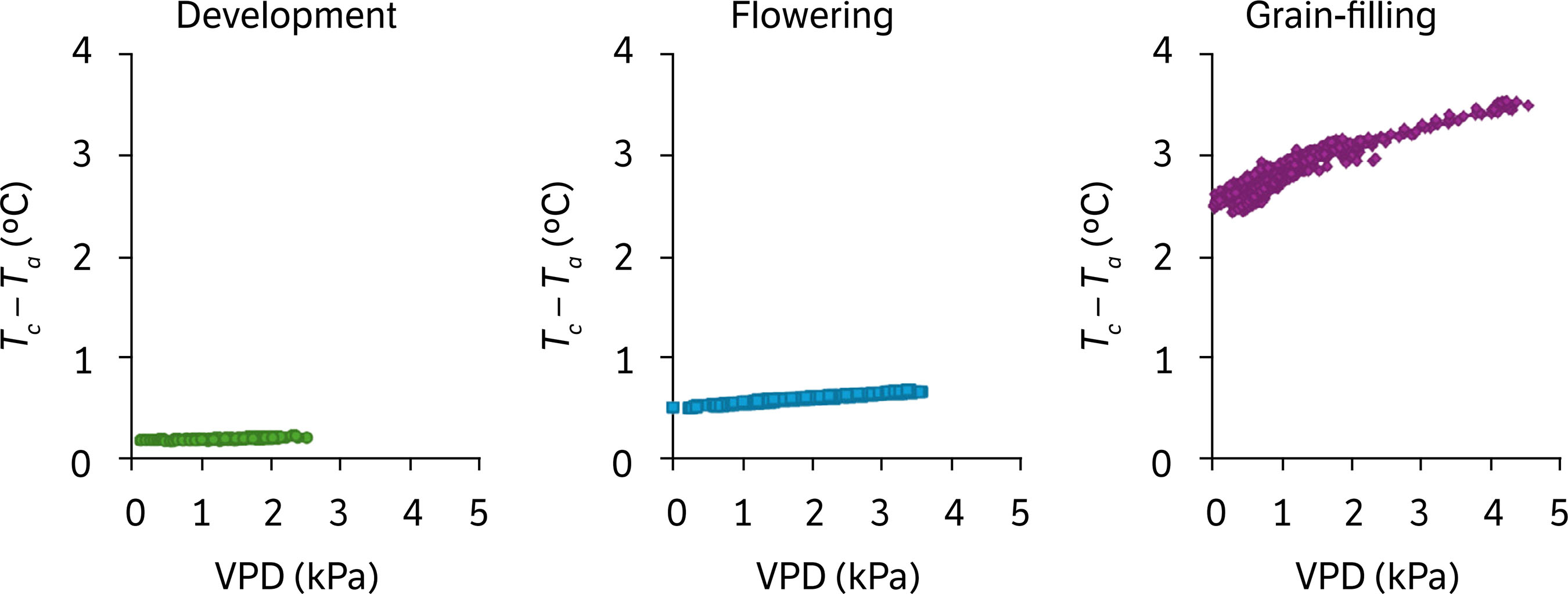
The canopy temperature was adjusted by incorporating canopy coverage and straw mulch temperature (Eq. 5). Figure 6 displays the resulting scatter plots. Since the ΔT model was derived with a limited amount of data, two additional filters were applied to avoid data extrapolation. The net radiation was set between 71 and 534 W·m^-2, and VPD values greater than 3 kPa were filtered out. As a result, all three phenological stages presented negative slopes. This outcome indicates that the procedure presented in this study was successful.

Figure 6
Canopy temperature (Eq. 5) minus air temperature (T _c – T _a) as a function of vapor pressure deficit: development, flowering, and grain-filling (first cycle). Data from 9 a.m. to 2 p.m. with wind speed, rainfall, net radiation, and vapor pressure deficit filters.

ANOVA was used to compare the difference between the canopy and air temperatures (T _c – T _a) in the datasets presented in Fig. 6. The test indicated that (T _c – T _a) varied significantly (p < 0.05) between any possible combination. Therefore, the NWSB was derived separately for each phenological stage (Fig. 7). Data averaging was also used to improve the goodness of fit. After sorting the VPD from the lowest to the highest value, a five-point moving average was applied to each dataset.

Figure 7
Non-water-stress baseline: development, flowering, and grain-filling (first cycle). A five-point moving average was applied to the data.

Table 5 presents the statistics for each NWSB illustrated in Fig. 7. Flowering and grain-filling had similar slopes but different intercepts. Both phenological stages exhibited an R2 value close to 0.8 and an RMSE of less than 0.9°C. Also, all their coefficients were statistically significant (p < 0.05). Regarding the development phase, the R² value was close to 0.7, and the RMSE was 1.2°C. The intercept was not statistically significant (p = 0.7), and its confidence interval contained zero.

Table 5
Statistics of the non-water-stress baseline for each phenological stage (first cycle).

Phenological stage		Coefficients	p-value	Lower 95%	Upper 95%	R2	RMSE
Development	a	0.10	0.7	-0.51	0.72	0.71	1.2
	b	-3.71	< 0.00001	-4.12	-3.30
Flowering	a	0.37	0.03	0.05	0.70	0.79	0.88
	b	-2.50	< 0.00001	-2.67	-2.33
Grain-filling	a	1.76	< 0.00001	1.59	1.93	0.78	0.87
	b	-2.71	< 0.00001	-2.85	-2.56

The upper limits of the difference between canopy and air temperature (T _c – T _a)_U were obtained using the NWSB coefficients (Eq. 8). Figure 8 shows (T _c – T _a)_U as a function of VPD for each phenological stage. A comparison of Fig. 8 and Table 5 reveals that the upper limit increased with the NWSB intercept.

Figure 8
The upper limit (T _c – T _a)_U, calculated with the non-water-stress baseline coefficients: development, flowering, and grain-filling (first cycle).

Crop water stress index

In the second cycle, the canopy coverage and straw mulch temperature were only considered for the development phase. The canopy coverage saturated at ~1 on the fifth day of flowering (34 DAP). After that, the canopy temperature was nearly equal to the temperature of the IRR sensor. The same wind speed and rainfall filters were applied to the second cycle data. However, the net radiation and VPD filters were only applied to the development data because of the ΔT model.

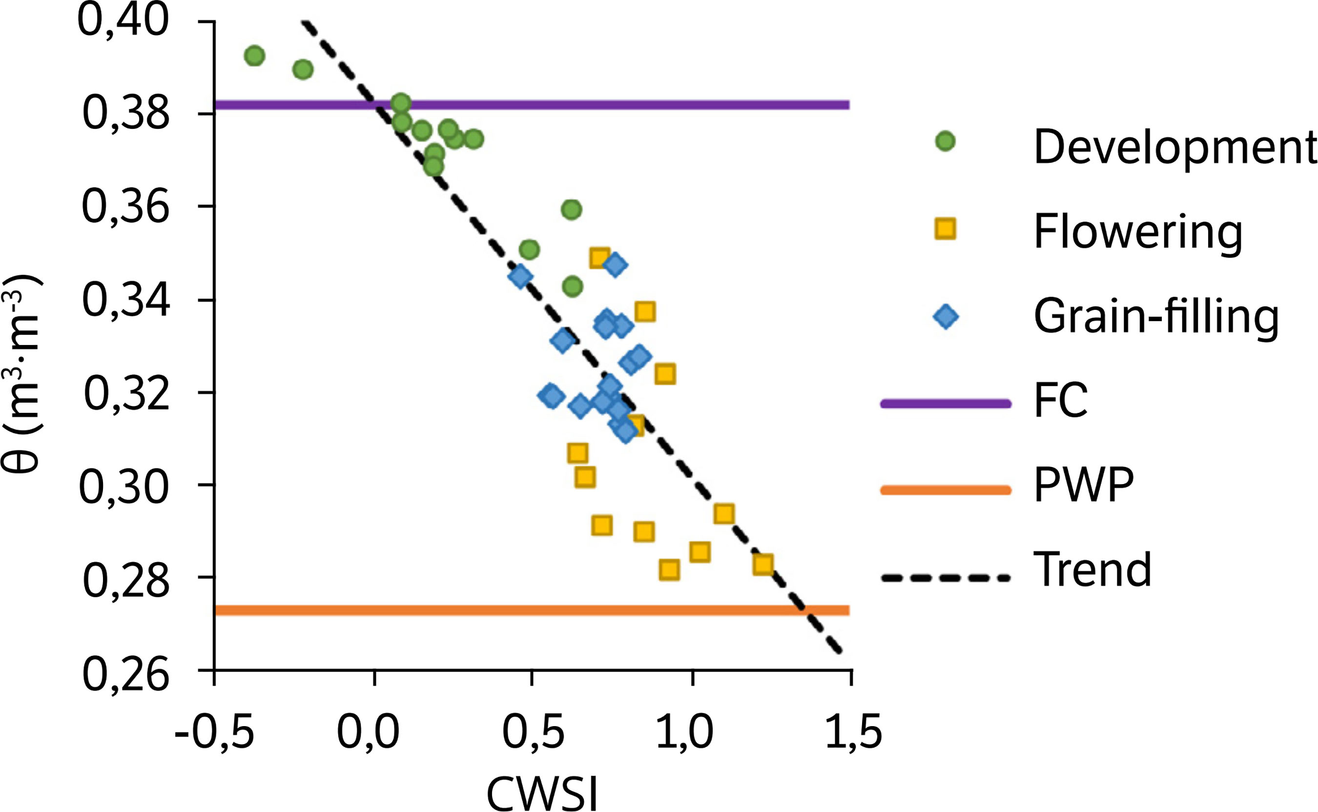
From the soil retention curve, the field capacity was 0.382 m³·m^-3, and the permanent wilting point was 0.273 m³·m^-3. Additionally, the soil water availability factor is 0.45 for common beans (ANA 2019). Thus, in the second cycle, water management was adequate during development, as shown in Fig. 9. However, water stress occurred during the other phenological stages of interest. It was severe during flowering and mild during grain-filling. Figure 9 also shows the box plots for the corresponding CWSI values. As expected, the CWSI average was the lowest for development and the highest for flowering.

Figure 9
Soil water content (θ) and crop water stress index (CWSI): development, flowering, and grain-filling (second cycle).

On the other hand, the CWSI values were not limited to the [0, 1] interval (Fig. 9). In fact, 18% of the CWSI values were negative and divided almost equally between development and grain-filling. Additionally, 24% of the CWSI values exceeded 1, with two-thirds corresponding to flowering. Negative values may indicate that the lower limit was too high, and values above 1 may indicate that the upper limit was too low. One possible reason was that the NWSB was derived using data from August to October, whereas the CWSI assessment used data from February to April.

The soil water content was averaged daily, and the data were organized into bins of 0.02 m³·m^-3 (Table 6). The soil water content remained close to field capacity for seven days during development. In contrast, the soil water content came close to the permanent wilting point for six days during flowering. For 17 days during grain-filling, the water content remained between 0.30 and 0.34 m³·m^-3

Table 6
Number of days and crop water stress index (CWSI) quartiles corresponding to different soil water content values, organized into bins of 0.02 m³·m^-3.

Soil water content (m3·m-3)	Number of days				CWSI
	Development	Flowering	Grain-filling		Q1	Q3
[0.28, 0.30]	0	6	1		0.44	1.35
(0.30, 0.32]	0	3	10		0.36	0.92
(0.32, 0.34]	0	2	7		0.49	1.06
(0.34, 0.36]	3	1	2		0.33	0.98
(0.36, 0.38]	7	0	0		-0.11	0.6
> 0.38	3	0	0		-0.79	0.2

Table 6 also displays the first and third quartiles of the CWSI for each water content bin. Those quartiles were used to trim the data before applying daily averages for the CWSI. Finally, the averaged soil water content was plotted against the trimmed and averaged CWSI (Fig. 10). The dashed line shows a clear trend, with an RMSE of 0.02 m³·m^-3 and an R² of 0.75. Figure 10 also shows the field capacity and permanent wilting point for reference.

Figure 10
Soil water content (θ) against crop water stress index (CWSI): development, flowering, and grain-filling (second cycle). Data trimming and data averaging were applied.

CONCLUSION

This study evaluated the feasibility of obtaining the NSWB and CWSI for bean phenological stages with low canopy coverage. The proposed procedure for adjusting canopy temperature produced interesting results. This procedure considers the IRR sensor measurement as the weighted mean of canopy and straw mulch temperatures, with the canopy coverage as the weighting factor. The canopy coverage was estimated using RGB images (first cycle) and the leaf area index (second cycle). The straw mulch temperature was estimated indirectly to avoid a division by the canopy coverage (f _c < 1). In future works, an IRR sensor shall be dedicated to measuring the straw mulch temperature to obtain a more robust estimation model.

Without the proposed procedure, the behavior of the scatter plots of the temperature difference against VPD did not correspond to the CWSI theory. The slope was positive in the development phase and null in flowering. After applying the proposed procedure, all scatter plots showed negative slopes, as expected. Thus, the proposed procedure was successful in adjusting the canopy temperature.

Quantitatively, the calculated CWSI produced points outside the expected range between 0 and 1. However, the result was promising qualitatively. After trimming and averaging the data, a clear trend was evident when the soil water content was plotted against the CWSI. In future works, CWSI maps shall be drawn using a thermographic camera once the upper and lower limits are established. Then, a map of estimated water content shall be derived from the CWSI.

ACKNOWLEDGMENTS

The authors thank the Divisão de Pesquisa e Desenvolvimento de Grãos e Fibras for providing space for data collection in the center-pivot area.

• How to cite:
  Góes, J. A., Prado, D. F. S., Pires, R. C. M., Chiorato, A. F. and Silveira, J. M. C. (2025). Crop water stress index of beans. Bragantia, 84, e20240235. https://doi.org/10.1590/1678-4499.20240235
• FUNDING
  Fundação de Apoio à Pesquisa Agrícola
  Grant No.: 1359
  Conselho Nacional de Desenvolvimento Científico e Tecnológico
  Grant No.: 136722/2023-7
  Fundação de Amparo à Pesquisa do Estado de São Paulo
  Grant Nos.: 2021/11762-5 and 2022/09319-9

DATA AVAILABILITY STATEMENT

The data supporting this study’s findings shall be available upon request.

REFERENCES

• [ANA] Agência Nacional de Águas (2019). Coeficientes técnicos de uso da água para a agricultura irrigada. Brasília: ANA.
• [ANA] Agência Nacional de Águas e Saneamento Básico (2021). Atlas irrigação: uso da água na agricultura irrigada. Brasília: ANA.
• Anderson, M. C., Neale, C. M. U., Li, F., Norman, J. M., Kustas, W. P., Jayanthi, H. and Chavez, J. (2004). Upscaling ground observations of vegetation water content, canopy height, and leaf area index during SMEX02 using aircraft and Landsat imagery. Remote Sensing of Environment, 92, 447-464. https://doi.org/10.1016/j.rse.2004.03.019
  » https://doi.org/10.1016/j.rse.2004.03.019
• Arantes, L. T., Arantes, B. H. T., Giongo, P. R., Ceccato, G. Z., Moraes, V. H., Saito, Y. K., Gomes, L. F. and Castro, A. C. O. (2021). Comportamento espectral e detecção de laranjeiras (Citrus sinensis L. Osbeck) com estresse hídrico, por meio de drone. Revista Brasileira de Geografia Física, 13, 3625-3635. https://doi.org/10.26848/rbgf.v13.07.p3625-3635
  » https://doi.org/10.26848/rbgf.v13.07.p3625-3635
• Ballester, C., Jiménez-Bello, M. A., Castel, J. R. and Intrigliolo, D. S. (2013). Usefulness of thermography for plant water stress detection in citrus and persimmon trees. Agricultural and Forest Meteorology, 168, 120-129. https://doi.org/10.1016/j.agrformet.2012.08.005
  » https://doi.org/10.1016/j.agrformet.2012.08.005
• Bellvert, J., Marsal, J., Girona, J., Gonzalez-Dugo, V., Fereres, E., Ustin, S. L. and Zarco-Tejada, P. J. (2016). Airborne thermal imagery to detect the seasonal evolution of crop water status in peach, nectarine and Saturn peach orchards. Remote Sensing, 8, 39. https://doi.org/10.3390/rs8010039
  » https://doi.org/10.3390/rs8010039
• Campbell, G. S. and Norman, J. M. (1998). The light environment of plant canopies. In G. S. Campbell and J. M. Norman (Eds.). An introduction to environmental biophysics (p. 247-278). New York: Springer. https://doi.org/10.1007/978-1-4612-1626-1
  » https://doi.org/10.1007/978-1-4612-1626-1
• Cunha, T. P. L., Mingotte, F. L. C., Carmeis Filho, A. C. A. C., Chiamolera, F. M., Lemos, L. B. and Fornasieri Filho, D. (2015). Agronomic performance of common bean in straw mulch systems and topdressing nitrogen rates in no-tillage. Revista Ceres, 62, 489-495. https://doi.org/10.1590/0034-737X201562050010
  » https://doi.org/10.1590/0034-737X201562050010
• Gonzalez-Dugo, V., Lopez-Lopez, M., Espadafor, M., Orgaz, F., Testi, L., Zarco-Tejada, P., Lorite, I. J. and Fereres, E. (2019). Transpiration from canopy temperature: Implications for the assessment of crop yield in almond orchards. European Journal of Agronomy, 105, 78-85. https://doi.org/10.1016/j.eja.2019.01.010
  » https://doi.org/10.1016/j.eja.2019.01.010
• Gonzalez-Dugo, V., Testi, L., Villalobos, F. J., López-Bernal, A., Orgaz, F., Zarco-Tejada, P. J. and Fereres, E. (2020). Empirical validation of the relationship between the crop water stress index and relative transpiration in almond trees. Agricultural and Forest Meteorology, 292-293, 108128. https://doi.org/10.1016/j.agrformet.2020.108128
  » https://doi.org/10.1016/j.agrformet.2020.108128
• Gonzalez-Dugo, V., Zarco-Tejada, P. J. and Fereres, E. (2014). Applicability and limitations of using the crop water stress index as an indicator of water deficits in citrus orchards. Agricultural and Forest Meteorology, 198-199, 94-104. https://doi.org/10.1016/j.agrformet.2014.08.003
  » https://doi.org/10.1016/j.agrformet.2014.08.003
• Han, M., Zhang, H., DeJonge, K. C., Comas, L. H. and Gleason, S. (2018). Comparison of three crop water stress index models with sap flow measurements in maize. Agricultural Water Management, 203, 366-375. https://doi.org/10.1016/j.agwat.2018.02.030
  » https://doi.org/10.1016/j.agwat.2018.02.030
• Idso, S. B., Jackson, R. D., Pinter, P. J., Reginato, R. J. and Hatfield, J. L. (1981). Normalizing the stress-degree-day parameter for environmental variability. Agricultural Meteorology, 24, 45-55. https://doi.org/10.1016/0002-1571(81)90032-7
  » https://doi.org/10.1016/0002-1571(81)90032-7
• Katimbo, A., Rudnick, D. R., DeJonge, K. C., Lo, T. H., Qiao, X., Franz, T. E., Nakabuye, H. N. and Duan, J. (2022). Crop water stress index computation approaches and their sensitivity to soil water dynamics. Agricultural Water Management, 266, 107575. https://doi.org/10.1016/j.agwat.2022.107575
  » https://doi.org/10.1016/j.agwat.2022.107575
• Laing, D. R., Jones, P. G. and Davis, J. H. C. (1984). Common bean (Phaseolus vulgaris L.). In P. R. Goldsworthy and N. M. Fisher (Eds.). The physiology of tropical field crops (p. 305-351). Wiley.
• Li, X., Duan, F., Hu, M., Hua, J. and Du, X. (2023). Weed density detection method based on a high weed pressure dataset and improved PSP net. IEEE Access, 11, 98244-98255. https://doi.org/10.1109/ACCESS.2023.3312191
  » https://doi.org/10.1109/ACCESS.2023.3312191
• Li, Y., Huang, Z., Cao, Z., Lu, H., Wang, H. and Zhang, S. (2020). Performance evaluation of crop segmentation algorithms. IEEE Access, 8, 36210-36225. https://doi.org/10.1109/ACCESS.2020.2969451
  » https://doi.org/10.1109/ACCESS.2020.2969451
• Luan, Y., Xu, J., Lv, Y., Liu, X., Wang, H. and Liu, S. (2021). Improving the performance in crop water deficit diagnosis with canopy temperature spatial distribution information measured by thermal imaging. Agricultural Water Management, 246, 106699. https://doi.org/10.1016/j.agwat.2020.106699
  » https://doi.org/10.1016/j.agwat.2020.106699
• Mariano, J. C. Q., Santos, G. O., Feitosa, D. G. and Hernandez, F. B. T. (2011). Sistema para manejo da agricultura irrigada – SIMAI (Computer software). Ilha Solteira: UNESP. Available at: http://clima.feis.unesp.br/smai.php Accessed on: August 28, 2025.
  » http://clima.feis.unesp.br/smai.php
• Monteith, J. L. (1969). Light interception and radiative exchange in crop stands. In J. D. Easting, F. A. Haskins, C. Y. Sullivan C. H. M. and Van Bavel (Eds.). Physiological aspects of crop yield (p. 89-116). Madison: American Society of Agronomy and Crop Science Society of America.
• O’Toole, J. C. and Hatfield, J. L. (1983). Effect of wind on the crop water stress index derived by infrared thermometry. Agronomy Journal, 75, 811-817. https://doi.org/10.2134/agronj1983.00021962007500050019x
  » https://doi.org/10.2134/agronj1983.00021962007500050019x
• Poblete-Echeverría, C., Espinace, D., Sepúlveda-Reyes, D., Zúñiga, M. and Sanchez, M. (2017). Analysis of crop water stress index (CWSI) for estimating stem water potential in grapevines: comparison between natural reference and baseline approaches. Acta Horticulturae, 1150, 189-194. https://doi.org/10.17660/ActaHortic.2017.1150.27
  » https://doi.org/10.17660/ActaHortic.2017.1150.27
• Sánchez-Piñero, M., Martín-Palomo, M. J., Andreu, L., Moriana, A. and Corell, M. (2022). Evaluation of a simplified methodology to estimate the CWSI in olive orchards. Agricultural Water Management, 269, 107729. https://doi.org/10.1016/j.agwat.2022.107729
  » https://doi.org/10.1016/j.agwat.2022.107729
• Siyal, A. W., Gerbens-Leenes, P. W. and Vaca-Jiménez, S. D. (2023). Freshwater competition among agricultural, industrial, and municipal sectors in a water-scarce country. Lessons of Pakistan’s fifty-year development of freshwater consumption for other water-scarce countries. Water Resources and Industry, 29, 100206. https://doi.org/10.1016/j.wri.2023.100206
  » https://doi.org/10.1016/j.wri.2023.100206
• Testi, L., Goldhamer, D. A., Iniesta, F. and Salinas, M. (2008). Crop water stress index is a sensitive water stress indicator in pistachio trees. Irrigation Science, 26, 395-405. https://doi.org/10.1007/s00271-008-0104-5
  » https://doi.org/10.1007/s00271-008-0104-5
• United Nations (2016). The Sustainable Development Goals Report 2016. New York: United Nations Publications.
• Van Genuchten, M. Th. (1980). A closed-form equation for predicting the hydraulic conductivity of unsaturated soils. Soil Science Society of America Journal, 44, 892-898. https://doi.org/10.2136/sssaj1980.03615995004400050002x
  » https://doi.org/10.2136/sssaj1980.03615995004400050002x
• Yin, W., Fan, Z., Hu, F., Fan, H., He, W., Zhao, C., Yu, A. and Chai, Q. (2023). No-tillage with straw mulching promotes wheat production via regulating soil drying-wetting status and reducing soil-air temperature variation at arid regions. European Journal of Agronomy, 145, 126778. https://doi.org/10.1016/j.eja.2023.126778
  » https://doi.org/10.1016/j.eja.2023.126778

Edited by

• Section Editor:
  Gabriel Constantino Blain https://orcid.org/0000-0001-8832-7734

Publication Dates

• Publication in this collection
  17 Oct 2025
• Date of issue
  2025

History

• Received
  15 Oct 2024
• Accepted
  18 Aug 2025