Comparative analysis between the XGBoost and Prophet models for the prediction of the ROTI ionospheric index: a case study in the Equatorial Ionization Anomaly region

Abstract:

Predicting ionospheric irregularities poses a significant challenge for applications that rely on real-time positioning accuracy using the GNSS. This work presents a comparative analysis between the Prophet and XGBoost models in the prediction of the ROTI index, using time series collected by the ITAI RBMC station, located in Foz do Iguaçu/PR, during the year 2024 (peak of solar cycle 25). This study contributes to the literature by providing a direct comparison between an additive statistical model and a gradient boosting algorithm for ROTI prediction in the Equatorial Ionization Anomaly region during solar maximum conditions. Both models were subjected to the same database and predictor variables. Training and validation were conducted through cross-validation specific to time series, utilizing the chronological division of the data and evaluating performance based on the RMSE, MAE, and R² metrics. The results obtained demonstrated that XGBoost outperformed Prophet in all analyzed metrics, indicating a greater capacity for adjustment and generalization. Statistical analysis of the residuals, including normality testing and non-parametric hypothesis tests, confirmed the robustness and consistency of the XGBoost predictions. However, we noted that the operational test window covered only 72 hours (1-3 October 2024), which constrained the generalizability of these results.

Keywords:
Ionosphere; XGBoost; Prophet; Prediction; Time Series

1. Introduction

Global Navigation Satellite Systems (GNSS) are integral tools for a wide range of modern applications, including air navigation, precision agriculture, and geodetic surveys, which require highly accurate positioning (Monico 2008). The performance of these systems, however, is significantly impacted by the ionosphere, a dynamic layer of the upper atmosphere whose variability can introduce delays and scintillations into signals. Such disturbances are particularly intense in low-latitude regions, including Brazil. This is largely due to the Equatorial Ionization Anomaly (EIA), which exacerbates the occurrence of ionospheric irregularities and complicates error mitigation (Pereira & Camargo 2017).

To quantify and monitor these phenomena, the Rate of TEC Index (ROTI) has established itself as a crucial metric, valued for its effectiveness in detecting rapid fluctuations in Total Electron Content (TEC) that compromise GNSS signal integrity (Pi et al. 1997). According to the classification proposed by Oladipo and Schuler (2013), average ROTI values below 0.4 TECU/min indicate background ionospheric conditions (absence of irregularities), values between 0.4 and 0.8 represent moderate irregularities, while values above 0.8 TECU/min denote severe disturbances. Therefore, the ability to accurately predict the ROTI index is of significant strategic importance for ensuring the reliability of critical operations. Traditional empirical models, such as the International Reference Ionosphere (IRI), although widely used, often exhibit limitations in capturing the abrupt and nonlinear patterns characteristic of ionospheric behavior during geomagnetic storms or periods of high solar activity (Bilitza 2001).

The state-of-the-art in ionospheric irregularity forecasting has been driven by the application of machine learning models, which demonstrate superior ability to capture the nonlinear dynamics of the ionospheric plasma. Salah et al. (2024) successfully implemented a Nonlinear AutoRegressive with eXogenous inputs (NARX) Neural Network to predict the ROTI index at the northern anomaly ridge in Egypt. Their study showed that including IRI model parameters as exogenous inputs significantly improves the model’s ability to learn about the behavior of the F layer. Similarly, Tete et al. (2024) employed a Feedforward Neural Network for the African region. They observed a significant increase in model accuracy when incorporating features extracted through wavelet decomposition, underscoring the importance of preprocessing and feature extraction from input data.

Complementing these approaches, other studies have investigated hybrid and spatially-aware architectures to further enhance predictive capabilities. Zhao et al. (2021) compared gradient boosting algorithms (XGBoost, LightGBM, and CatBoost) for predicting the day-to-day occurrence of ionospheric scintillation at low latitudes, demonstrating the effectiveness of ensemble tree-based methods in this domain. From a spatiotemporal perspective, Liu et al. (2021) used a Convolutional Long Short-Term Memory (convLSTM) model to predict the evolution of 2D ROTI maps at high latitudes during geomagnetic storms. They demonstrated that a custom loss function can improve the model’s ability to predict spatial structures of irregularities up to 60 minutes in advance.

Taken together, these studies indicate a clear trend toward using multi-source data and increasingly sophisticated models to provide more accurate and timely forecasts of ionospheric irregularities. Despite these advances, direct comparisons between different modeling paradigms, such as neural networks and decision-tree-based ensemble algorithms, remain an area of ​​active research. Although ensemble models show promise, understanding the strengths and limitations of their individual components is essential. As noted by Makridakis et al. (2018), the relative performance of statistical and machine learning methods depends heavily on the characteristics of the data. While Zhao et al. (2021) demonstrated the potential of gradient boosting algorithms for ionospheric scintillation prediction, the isolated performance of XGBoost against a purely statistical model for ROTI prediction has not yet been evaluated.

This study, therefore, seeks to present a comparative analysis between two models representing fundamentally different forecasting paradigms: Prophet, an additive statistical model designed for interpretability and the handling of strong seasonality (Taylor & Letham 2018), and XGBoost, a high-performance gradient boosting algorithm recognized for its robustness in complex and nonlinear scenarios (Chen & Guestrin 2016). The rationale for selecting these two models lies in their contrasting approaches to time series forecasting: Prophet decomposes the series into interpretable components (trend, seasonality, holidays), while XGBoost constructs an ensemble of decision trees that can capture arbitrary nonlinear interactions between features. The handling of the holidays term in the present study is detailed in Section 2.3. This contrast allows for a direct assessment of whether the complex, non-stationary dynamics of ionospheric irregularities are better modeled by an interpretable additive framework or by a flexible nonlinear learner.

Using a time series of the ROTI index from the ITAI station (Foz do Iguaçu, Paraná) of the RBMC (Brazilian Network for Continuous Monitoring of GNSS Systems), collected during 2024 (period corresponding to the peak of solar cycle 25), this article aims to: measure the predictive performance of both models under identical data and attribute engineering conditions; identify the capabilities and limitations of each approach in predicting ionospheric irregularities during a solar maximum; and provide subsidies for the selection of suitable models for operational ionospheric monitoring systems. To the best of the authors’ knowledge, this represents the first direct comparison between an additive statistical model and a gradient boosting algorithm for ROTI prediction in the EIA region.

2. Methodology

The methodology adopted in this study was structured to ensure the robustness and reproducibility of the comparative analysis. The steps include describing the data source, preprocessing and feature engineering, specifying the predictive models, and finally, the training protocol and performance evaluation.

2.1 Database

The ROTI data used in this work were generated by the Ion_Index computational application (Pereira & Camargo 2017), which processes GNSS observables collected by RBMC stations. For this case study, the ITAI station (Figure 1) was selected, located in Foz do Iguaçu, Paraná (Geodetic Latitude: 25° 25’ 14.44” S, Geodetic Longitude: 54° 35’ 17.85” W; Geomagnetic Latitude: 15° 34’ 48” S). The choice of this station is strategic, as its geographic position is under the direct influence of the Equatorial Ionization Anomaly (EIA), a region characterized by intense ionospheric variability. The time series analyzed spans the period from January 1 to October 31, 2024, a year marked by high solar activity.

Figure 1:
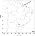
Location of RBMC ITAI station. Latitude and Longitude are expressed in degrees South and West, respectively.

2.2 Data Preparation and Attribute Engineering

The ROTI time series, originally with one-second resolution, was aggregated into hourly averages. In the context of ionospheric forecasting, short-term prediction typically encompasses horizons ranging from one hour to one day (Cander 2015; Zolesi & Cander 2014). The present study adopts an extended short-term horizon of 72 hours, which is relevant for operational planning of GNSS-dependent activities such as Unmanned Aerial Vehicle (UAV) missions and precision agriculture, where the aim is to anticipate time windows of greater ionospheric instability rather than reacting to instantaneous scintillations. Although ROTI is a metric designed to detect rapid variations, hourly aggregation was adopted in this study for a specific purpose: to develop a forecasting model focused on these operational trends. Furthermore, the aggregation process acts as a filter, mitigating high-frequency noise and thereby improving the stability of the series for modeling purposes.

From the hourly time series, a comprehensive feature engineering process was performed to enrich the data set used in predictive modeling. In total, additional features were generated, encompassing different dimensions of temporal and statistical variability.

Initially, cyclical temporal attributes were constructed to capture seasonal patterns present in the data. To this end, transformations based on sine and cosine functions were applied to the hour, day of the week, day of the month, and day of the year variables, taking into account their respective periods. These transformations followed the formulation and where v corresponds to the value of the temporal variable and P to the associated period (e.g., 24 for hours).

Furthermore, lag features were incorporated, consisting of ROTI index values ​​recorded from 1 to 24 hours before the forecast time. The selection of this lag range was guided by an autocorrelation analysis of the hourly ROTI series (Box et al. 2015). The Autocorrelation Function (ACF) revealed strong temporal dependence at lag-1 (r = 0.84) and a prominent secondary peak at lag-24 (r = 0.81), reflecting the well-known diurnal cycle of ionospheric variability. The Partial Autocorrelation Function (PACF) confirmed lag-1 (r = 0.84) and lag-24 (r = 0.26) as the most significant individual predictors. These results justify the inclusion of lags spanning the full 24-hour diurnal cycle, as they capture both the short-term persistence and the daily periodicity of ionospheric irregularities. Additionally, statistics derived from moving windows, including means, standard deviations, minimum and maximum values, were calculated at intervals of 3, 6, 12, 24, and 48 hours.

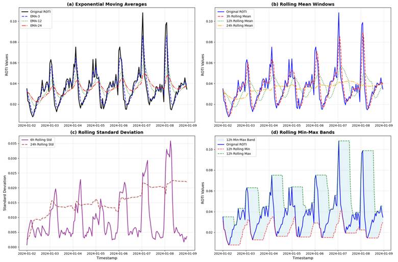
Finally, to represent trend and smoothing aspects of the series, first- and twenty-fourth-order differences, as well as exponential moving averages, were added. This diverse set of attributes aimed to enhance the models’ ability to capture the complex dynamics of the phenomenon under analysis. Figure 2 visually illustrates a subset of these variables, demonstrating how moving averages, standard deviations, and minimum-maximum bands capture the trend and local variability of the original ROTI series.

Figure 2:
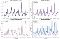
Examples of features generated through time series engineering from the ROTI data. The panels illustrate: (a) Exponential Moving Averages (EMA) with varying smoothing windows; (b) 6, 12, and 24-hour Simple Moving Averages (Rolling Mean); (c) Rolling Standard Deviation to capture local volatility; and (d) 12-hour Rolling Min-Max Bands, which delineate the local amplitude of the series.

To evaluate model performance and prevent future data leakage, the dataset was partitioned using a time series validation protocol. Records from January 1 to September 30, 2024, were designated as the development set. This set was subsequently split into 80% for training and 20% for validation. While optimal splitting ratios depend on the signal-to-noise ratio (Hastie et al. 2009), this proportion was selected to ensure sufficient data for the complex model learning while maintaining a representative validation set. The model tuning and hyperparameter optimization were performed through TimeSeriesSplit cross-validation with ten folds, preserving the temporal ordering of observations to prevent data leakage. Although Bergmeir and Benitez (2012) demonstrated that cross-validation techniques can be effectively applied to time series data, a sequential splitting strategy was adopted as a conservative approach to ensure strict chronological separation between training and validation sets. According to Kohavi (1995), ten-fold cross-validation provides an optimal balance between bias and variance for model selection. The values reported as ‘Training’ performance in Table 1 correspond to the average of the validation metrics (inference on unseen fold data) obtained across these ten iterations, ensuring a robust assessment of the model’s stability.

Furthermore, in accordance with the study’s operational focus, a subsequent, continuous period corresponding to the first 72 hours of October 2024 was isolated and reserved as a final test set. This approach follows the out-of-sample evaluation framework recommended by Tashman (2000) for time series forecasting, where a contiguous holdout period preserves the temporal structure of the data. This specific time window was selected to validate the model’s performance within a typical short-term operational forecasting horizon, simulating a real-world scenario where operators require accurate stability predictions for the upcoming days. This set was not used in any training or tuning stage, serving exclusively for the final evaluation of the models’ generalization ability on unseen data.

2.3 Predictive Models

Two distinct models were comparatively evaluated: Prophet, a statistical model, and XGBoost, a machine learning model. Both were trained and tested with the same set of attributes, ensuring methodological parity.

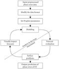
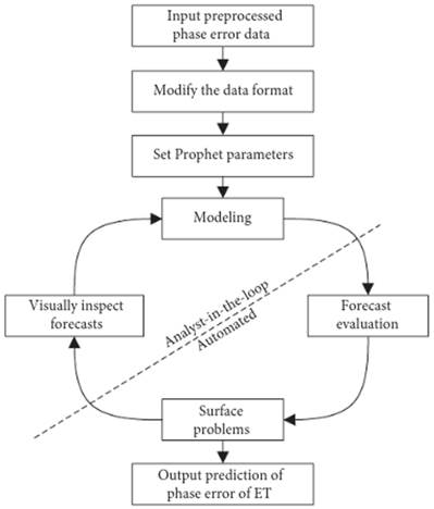
The Prophet model, developed by Taylor and Letham (2018), stands out for its additive approach, which decomposes the series into components, including trend and seasonality. The trend is modeled by a piecewise linear function or a logistic growth curve, with change points that capture changes in the series’ behavior. Seasonality, in turn, is modeled through Fourier series, allowing for the flexible capture of multiple periodic patterns, such as daily and annual cycles. The main advantage of Prophet lies in the interpretability of its parameters, facilitating an “analyst-in-the-loop” approach to modeling. Figure 3 illustrates this workflow, showing how raw data is decomposed into trend, seasonal, and residual components, which are then recombined to generate the final forecast.

The Prophet framework also supports an optional holidays component to model country-specific calendar events that may introduce localized impulse-like effects on the series. In the present study, however, no holidays were specified in the model configuration, since ionospheric variability is governed by geophysical and solar forcing rather than by civil-calendar events; including civil holidays as regressors would not be physically meaningful for the ROTI series. The holidays term is therefore identically zero throughout the forecast window and does not contribute to the additive decomposition. Consequently, the residual component shown in Figure 3 contains only the variability that is not captured by the trend and seasonal components and is not contaminated by a holidays contribution.

Figure 3:
Flowchart of Prophet model prediction.

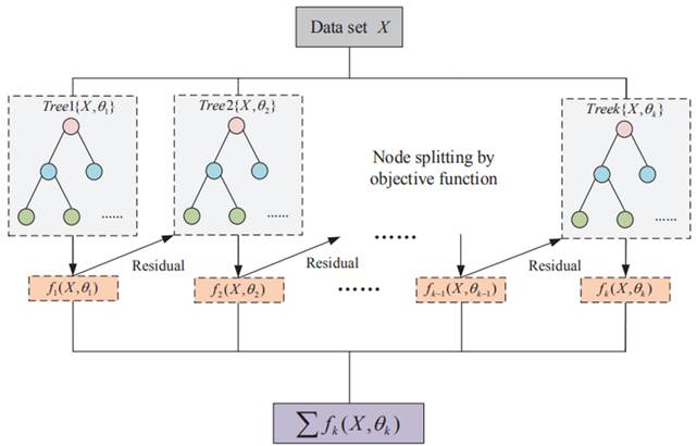
For prediction problems that can be structured as regression tasks, XGBoost (eXtreme Gradient Boosting) is a gradient tree boosting algorithm widely recognized for its high performance and scalability. Developed by Chen and Guestrin (2016), XGBoost stands out for its regularized learning objective, which penalizes model complexity to avoid overfitting. The system incorporates crucial optimizations, such as a sparsity-aware algorithm that efficiently handles missing data, and system optimizations that enable parallel, distributed, and out-of-core computing, making it viable for massive datasets. Figure 4 illustrates this iterative process, where each new tree is trained to correct the residual errors of the ensemble, with the final prediction being the sum of all individual tree contributions.

Figure 4:
Flowchart of XGBoost.

2.4 Model Evaluation

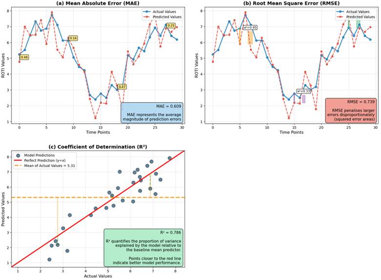
The performance of the models was evaluated using three metrics widely recognized in the time series and ionospheric prediction literature (Salah et al. 2024; Tete et al. 2024; Natras et al. 2022): Root Mean Square Error (RMSE), Mean Absolute Error (MAE), and Coefficient of Determination (R ² ). These metrics offer complementary perspectives on predictive accuracy (Willmott & Matsuura 2005): RMSE penalizes larger errors more severely, making it sensitive to outliers; MAE provides an unambiguous measure of average error magnitude; and R² quantifies the proportion of variance explained by the model.

The metrics are defined mathematically as follows. The Root Mean Square Error (RMSE) is calculated by:

$RMSE=\sqrt{\frac{1}{n}\sum _{i=1}^n{\left(y_i-{\widehat{y}}_i\right)}^2}$ (1)

The Mean Absolute Error (MAE) is given by:

$MAE=\frac{1}{n}\sum _{i=1}^n\left|y_i-{\widehat{y}}_i\right|$ (2)

And the Coefficient of Determination (R ² ) is expressed as:

$R^2=1-\frac{{\sum }_{i=1}^n{\left(y_i-{\widehat{y}}_i\right)}^2}{{\sum }_{i=1}^n{\left(y_i-\stackrel{-}{y}\right)}^2}$ (3)

Where n is the number of observations, y _i represents the observed value, $\widehat{y_i}$ is the predicted value, and $\stackrel{-}{y}$ is the mean of the observed values.

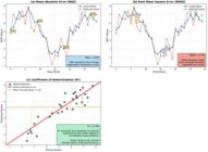
Figure 5 provides a conceptual illustration of how each of these metrics measures predictive performance: (a) RMSE, which emphasizes large deviations; (b) MAE, which treats all errors equally; and (c) R ² , which measures the goodness-of-fit relative to the mean.

Figure 5:
Conceptual illustration of the performance evaluation metrics.

To assess whether the residuals from the training and test phases differ significantly, indicating potential overfitting, a hypothesis test was applied to compare the distributions of residual errors. Prior to selecting the appropriate test, the normality of the residual distributions was verified using the Shapiro-Wilk test (Shapiro & Wilk 1965), which is recommended as one of the most powerful tests for assessing normality assumptions (Ghasemi & Zahediasl 2012). When the normality assumption is satisfied, the Student’s t-test for independent samples is applied; otherwise, the non-parametric Mann-Whitney U test is employed, which does not require distributional assumptions and is suitable for comparing two independent groups. In both cases, a significance level of alpha = 0.05 is adopted.

3. Results and Discussions

This section presents and analyzes the results obtained during the training and testing of the Prophet and XGBoost models in predicting the ROTI index. Section 3.1 analyzes the models’ performance during the cross-validation training phase, focusing on the stability and generalization capacity of each model across the ten temporal folds. Section 3.2 evaluates the models’ performance on the independent 72-hour test set, providing a realistic assessment of their operational forecasting capability. Finally, Section 3.3 consolidates the overall performance comparison through a summary table, visual analysis, and statistical hypothesis testing of the residuals.

3.1 Performance during training

During the training phase, conducted through cross-validation with ten temporal divisions, both models exhibited stable performance, albeit with varying responses to variations in the ROTI time series. The XGBoost model obtained an average RMSE value of 0.0164 and an MAE of 0.0115, demonstrating low error dispersion and high generalization capacity. Its average coefficient of determination (R²) was 0.8142, indicating good explanatory power for the variability observed in the data.

On the other hand, the Prophet model showed inferior performance under the same conditions. The average RMSE was 0.0250, while the MAE reached 0.0168. The average R² value was 0.7155, suggesting a lower capacity to capture the variability of the series compared to XGBoost. These results indicate that, despite Prophet’s ability to model regular seasonal patterns, its performance is limited when faced with abrupt fluctuations and nonlinear patterns present in the ROTI index.

To contextualize the practical significance of these differences, it is important to consider the scale of the ROTI index. According to the classification by Oladipo and Schuler (2013), averaged ROTI values below 0.4 TECU/min indicate background ionospheric conditions. The RMSE values obtained by XGBoost (0.0164 TECU/min) and Prophet (0.0250 TECU/min) are well below this threshold, indicating that both models achieve errors that are an order of magnitude smaller than the boundary between background and disturbed conditions. Despite both being well below the disturbance threshold, the gap between the two models is substantial, with Prophet’s training RMSE markedly higher than XGBoost’s, indicating a meaningful improvement in predictive accuracy when using the gradient boosting approach. Similar performance advantages of gradient boosting methods over simpler approaches have been reported in other ionospheric studies, such as Zhao et al. (2021) for scintillation prediction and Natras et al. (2023) for VTEC forecasting.

3.2 Performance on the test set

In the test set, corresponding to the 72-hour operational horizon (October 1 to 3, 2024), the XGBoost model demonstrated superior performance, with an RMSE of 0.0094, an MAE of 0.0077, and an R² of 0.8569. While the statistical consistency of the model was established through the extensive cross-validation process (Section 3.1), this final test confirms the model’s capability to deliver accurate predictions specifically within the short-term forecasting window required for GNSS operational planning. These values confirm its predictive robustness in a realistic deployment scenario.

The Prophet model, in turn, yielded an RMSE of 0.0234, an MAE of 0.0174, and an R² of 0.1238 within the same interval. Despite maintaining functional performance, the difference between the models is substantial, especially in the absolute error and root mean square error metrics. Prophet’s MAE and RMSE were 126.0% and 148.9% higher than those of XGBoost, respectively, indicating that Prophet’s errors are more than double those of XGBoost. Regarding the coefficient of determination, XGBoost explained 85.7% of the data variance (R² = 0.8569), whereas Prophet explained only 12.4% (R² = 0.1238), representing a difference of 0.7331 in absolute terms.

The residual analysis reveals essential aspects of the models’ behavior: XGBoost presents a mean residual close to zero (-0.000038) with a standard deviation of 0.0094, while Prophet exhibits systematic bias with a mean residual of -0.0097 and greater variability (standard deviation of 0.0212). This lower error variability in XGBoost indicates greater consistency in predictions, a crucial aspect for operational applications.

These results highlight the limitations of the Prophet additive statistical model in handling the nonlinear complexity of the ROTI series in short-term forecasting scenarios, while reinforcing the applicability of XGBoost in operational environments that demand continuous forecasts with a high degree of accuracy and reliability.

3.3 Performance analysis of the models

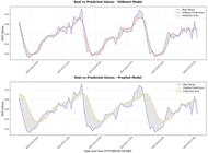
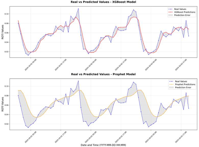
Table 1 summarizes the main results obtained by both models. In all cases, the XGBoost model presented lower RMSE and MAE values, and higher coefficients of determination, indicating its superiority in terms of predictive performance. Figure 6 shows the prediction plot against the observed values of the XGBoost and Prophet models, respectively.

Figure 6 presents the actual versus predicted values for both models during the 72-hour test period. The figure clearly illustrates the contrasting behavior of the two approaches: the XGBoost predictions closely track the actual ROTI variations, capturing both the diurnal oscillations and their amplitudes with high fidelity. In contrast, the Prophet predictions exhibit a systematic negative bias and fail to reproduce the amplitude of the observed fluctuations, resulting in larger shaded error areas. The difference in the area between the predicted and actual curves visually confirms the quantitative metrics presented in Table 1.

Table 1:
Comparison of the performance metrics of the Prophet and XGBoost models in the training and testing phases.

Phase	Model	RMSE	MAE	R²
Training	Prophet	0.0250	0.0168	0.7155
	XGBoost	0.0164	0.0115	0.8142
Test Set (72h Operational Horizon)	Prophet	0.0234	0.0174	0.1238
	XGBoost	0.0094	0.0077	0.8569

Figure 6:
Actual versus predicted values for the Prophet and XGBoost models.

The advantage of XGBoost is attributed to its ability to model complex, nonlinear relationships and the robustness of the boosting process, which allows for efficient adaptation even in the face of sudden oscillations in the time series. Prophet, although suitable for series dominated by regular seasonal patterns, proved to be limited when faced with the demands of ROTI forecasting, which involves both periodic variations and erratic behavior.

The distribution of the residuals was assessed for both models to verify the consistency of the errors and identify potential signs of overfitting. In the case of XGBoost, the residuals presented a symmetrical and centered distribution close to zero, with low dispersion. Prior to the hypothesis testing, the Shapiro-Wilk normality test was applied to the residuals of both models. The results indicated that the residual distributions deviate significantly from normality for both XGBoost (W = 0.910, p < 0.001) and Prophet (W = 0.935, p = 0.001). This deviation from normality is consistent with the physical nature of the ROTI series and can be attributed to three main factors. First, heavy-tailed events: sporadic ionospheric scintillations and plasma bubbles, particularly frequent in the EIA region during solar maximum, produce occasional large excursions in the observed series that propagate into the residuals and thicken the tails of their distribution (Pi et al. 1997; Pereira & Camargo 2017). Second, right-skewness ROTI is bounded below by zero and exhibits brief, high-amplitude peaks rather than symmetric oscillations around a mean, which biases the residual distribution and prevents it from being symmetric. Third, diurnal heteroscedasticity residual variance is markedly higher in the post-sunset sector of the EIA, where Equatorial Plasma Bubbles (EPBs) and irregularities preferentially develop (Salah et al. 2024); this regime-dependent variance further removes the residuals from a single Gaussian distribution. These features violate the i.i.d.-Gaussian assumption of the Student’s t-test and motivate the adoption of the non-parametric Mann-Whitney U test for the subsequent comparison of training and test residuals. Given this violation of the normality assumption, the non-parametric Mann-Whitney U test was adopted instead of the Student’s t-test, as recommended by Ghasemi and Zahediasl (2012).

For XGBoost, the Mann-Whitney U test applied between the absolute training and test residuals yielded a p-value well above the significance threshold of 0.05, indicating no statistically significant difference between the two sets. This suggests robustness and predictive stability, with no evidence of overfitting.

For Prophet, the residuals presented greater variability, with the presence of systematic patterns in some validation periods, which may indicate limitations of the model in adjusting to the specific oscillations of the ROTI series. The Mann-Whitney U test applied to this model indicated a p-value below the threshold of 0.05, signaling a statistically significant difference between the training and test errors, which may be related to the structural rigidity of the model in relation to the dynamics of the series.

4. Final Considerations

This study presents a comparative analysis of the Prophet and XGBoost models for predicting the ROTI index, utilizing data from the ITAI station throughout 2024. Both models were trained under identical input conditions, utilizing time series lags, seasonal components derived from trigonometric transformations, and moving averages. The evaluation was performed via time-series-specific cross-validation and subsequent testing on a holdout dataset.

The results demonstrated the superior performance of the XGBoost model across all metrics analysed. XGBoost yielded a lower Mean Absolute Error (MAE), a lower Root Mean Square Error (RMSE), and a higher Coefficient of Determination (R²) compared to Prophet, thereby demonstrating a greater capacity to capture the non-linear patterns and abrupt oscillations typical of ionospheric dynamics in regions under the influence of the Equatorial Ionization Anomaly. Statistical analysis of the residuals, using the Shapiro-Wilk normality test followed by the non-parametric Mann-Whitney U test, confirmed the consistency of XGBoost’s performance, with no evidence of overfitting, reinforcing its suitability for the problem at hand.

Conversely, whilst Prophet demonstrated stability in modelling seasonal components and trends, its additive structure proved limited when confronted with the complexity of the ROTI time series, resulting in a greater dispersion of errors and a lower explanation of the observed variance. Nevertheless, its application offers an interpretable and readily adjustable baseline, which can be useful in operational contexts with less structural variability.

These findings are consistent with the theoretical expectation that ensemble tree-based methods outperform additive statistical models in the presence of strong nonlinearity and non-stationarity, as discussed in the broader machine learning forecasting literature (Hastie et al. 2009; Makridakis et al. 2018). The dominance of XGBoost across all metrics suggests that the ROTI series, particularly during solar maximum, exhibits dynamics that are better captured by flexible nonlinear learners than by decomposition-based approaches.

The out-of-sample test set in this study is restricted to a 72-hour window (1-3 October 2024) within the peak of solar cycle 25. This window was chosen to match the operational forecasting horizon relevant for GNSS-dependent activities such as UAV missions and precision agriculture (Tashman 2000; Cander 2015), but is not by itself sufficient to characterize model behavior under the full range of ionospheric regimes including solar minimum conditions, severe geomagnetic storms, distinct seasons of the year, and other longitudinal sectors. Furthermore, the analysis is restricted to a single RBMC station (ITAI). Accordingly, the quantitative advantage of XGBoost over Prophet reported here should be interpreted as evidence for the studied window and station, and not as a universal claim regarding ionospheric forecasting in general. Extending the evaluation to additional periods of the solar cycle, to multiple RBMC stations, and to disturbed geomagnetic intervals constitutes a necessary follow-up to establish the broader operational applicability of the approach.

This comparison contributes to the literature by providing quantitative evidence on the suitability of different modelling paradigms for predicting ionospheric irregularities in real-time. The ability to predict periods of strong ionospheric instability in advance is crucial for GNSS applications that are sensitive to timing and signal reliability. Sectors such as Precision Agriculture, Air Navigation, Mining, and Structural Monitoring can directly benefit from accurate forecasts, using this information to optimize processes and anticipate critical operational decisions. Building on the limitations noted above, future work could therefore extend this study in several directions, including: the investigation of hybrid approaches that combine the interpretability of statistical models with the generalisation power of machine learning algorithms; the incorporation of additional variables, such as geophysical parameters and solar indices; and the expansion of the analysis to include data from multiple RBMC stations and across different periods of the solar cycle, to validate the models’ robustness under diverse spatial and geomagnetic conditions.

ACKNOWLEDGEMENT

NORTE project funded by agreement ITAIPU-UTFPR-FUNTEF, process number 4500069287-3793-1-14077-5.

REFERENCES

• Bergmeir, C., & Benitez, J. M. (2012). On the use of cross-validation for time series predictor evaluation. Information Sciences, 191, 192-213.
• Bilitza, D. (2001). International reference ionosphere 2000. Radio Science, 36(2), 261-275.
• Box, G. E. P., Jenkins, G. M., Reinsel, G. C., & Ljung, G. M. (2015). Time Series Analysis: Forecasting and Control (5th ed.). Wiley.
• Cander, Lj. R. (2015). Forecasting foF2 and MUF(3000)F2 ionospheric characteristics - A challenging space weather frontier. Advances in Space Research, 56(9), 1973-1981.
• Chen, T., & Guestrin, C. (2016). XGBoost: A scalable tree boosting system. In Proceedings of the 22nd ACM SIGKDD International Conference on Knowledge Discovery and Data Mining (pp. 785-794).
• Ghasemi, A., & Zahediasl, S. (2012). Normality Tests for Statistical Analysis: A Guide for Non-Statisticians. International Journal of Endocrinology and Metabolism, 10(2), 486-489.
• Guo, R., Zhao, Z., Wang, T., Liu, G., Zhao, J. and Gao, D. (2020). Degradation State Recognition of Piston Pump Based on ICEEMDAN and XGBoost. Applied Sciences, 10(18), p.6593.
• Hastie, T., Tibshirani, R., & Friedman, J. (2009). The Elements of Statistical Learning: Data Mining, Inference, and Prediction (2nd ed.). New York: Springer.
• Kohavi, R. (1995). A study of cross-validation and bootstrap for accuracy estimation and model selection. In Proceedings of the 14th International Joint Conference on Artificial Intelligence (Vol. 2, pp. 1137-1143).
• Liu, Z., Morton, Y. T., & Liu, Y. (2021). A Convolutional Long Short-Term Memory Network for Ionospheric Scintillation Forecasting. In Proceedings of the 34th International Technical Meeting of the Satellite Division of The Institute of Navigation (ION GNSS+ 2021) (pp. 2685-2696).
• Makridakis, S., Spiliotis, E., & Assimakopoulos, V. (2018). Statistical and Machine Learning forecasting methods: Concerns and ways forward. PLoS ONE, 13(3), e0194889.
• Monico, J. F. G. (2008). Posicionamento pelo GNSS: descricao, fundamentos e aplicacoes Editora Unesp.
• Natras, R., Soja, B., & Schmidt, M. (2022). Ensemble machine learning of Random Forest, AdaBoost and XGBoost for vertical total electron content forecasting. Remote Sensing, 14(15), 3547.
• Natras, R., Soja, B., & Schmidt, M. (2023). Uncertainty Quantification for Machine Learning-Based Ionosphere and Space Weather Forecasting. Space Weather, 21, e2023SW003483.
• Oladipo, O. A., & Schuler, T. (2013). Equatorial ionospheric irregularities using GPS TEC derived index. Journal of Atmospheric and Solar-Terrestrial Physics, 92, 78-82.
• Pereira, V. A. S., & Camargo, P. O. (2017). Brazilian active GNSS networks as systems for monitoring the ionosphere. GPS Solutions, 21(3), 1013-1025.
• Pi, X., Mannucci, A. J., Lindqwister, U. J., & Ho, C. M. (1997). Monitoring of global ionospheric irregularities using the worldwide GPS network. Geophysical Research Letters, 24(18), 2283-2286.
• Salah, H. M., Babatunde, R., Okoh, D., Youssef, M., & Mahrous, A. (2024). Machine learning approach for prediction of ionospheric irregularities on ROTI index over the Northern anomaly crest in Egypt during solar cycle 24. Advances in Space Research , 74(4), 1810-1827.
• Shapiro, S. S., & Wilk, M. B. (1965). An analysis of variance test for normality (complete samples). Biometrika, 52(3-4), 591-611.
• Tashman, L. J. (2000). Out-of-sample tests of forecasting accuracy: an analysis and review. International Journal of Forecasting, 16(4), 437-450.
• Taylor, S. J., & Letham, B. (2018). Forecasting at scale. The American Statistician, 72(1), 37-45.
• Tete, S., Otsuka, Y., Zahra, W. K., & Mahrous, A. (2024). Machine learning approach for ionospheric scintillation prediction on ROTI parameter over the African region during solar cycle 24. Advances in Space Research , 74(12), 6325-6342.
• Willmott, C. J., & Matsuura, K. (2005). Advantages of the mean absolute error (MAE) over the root mean square error (RMSE) in assessing average model performance. Climate Research, 30, 79-82.
• Ye, Y., Yang, A., Wu, Y., Hu, C., Li, M., Li, Y. and Deng, X. (2020). Short-Term Prediction of Electronic Transformer Error Based on Intelligent Algorithms. Journal of Control Science and Engineering, 2020, pp.1-9.
• Zhao, X., Li, G., Xie, H., et al. (2021). The Prediction of Day-to-Day Occurrence of Low Latitude Ionospheric Strong Scintillation Using Gradient Boosting Algorithm. Space Weather , 19(12), e2021SW002884.
• Zolesi, B., & Cander, Lj. R. (2014). Ionospheric Prediction and Forecasting Springer.

• DATA AVAILABILITY
  The datasets generated and analyzed during the current study are available from the corresponding author on reasonable request.

• Edited by
  Silvana Philippi Camboim e Daniele Barroca Marra Alves.

Data availability

The datasets generated and analyzed during the current study are available from the corresponding author on reasonable request.

Publication Dates

• Publication in this collection
  27 July 2026
• Date of issue
  2026

History

• Received
  06 Oct 2025
• Accepted
  21 May 2026