Novel programming pipeline for herbicide resistance prediction

Abstract

Background  Weeds evolve resistance to specific herbicide Mode of Actions (MoAs) through repeated herbicide use. Delaying herbicide resistance is a primary area of concern because there are a limited number of herbicide MoAs remaining.

Objective  The objective of this study was to create a generic model on weed resistance when various management practices are used. Academic herbicide resistant modeling tools have been developed to integrate knowledge about weed biology (species specific), genetics, weed management (herbicide dose response, herbicide rotation) because interactions may not always be intuitive. A variety of other interacting factors such as seed bank density, cropping system, and the initial resistant allele frequency in weed populations contribute to this dilemma.

Methods  Methods used provide details about a weed resistance model, along with representative results when two experimental herbicides with similar MoA are simulated for potential weed resistance over time to provide the ability to prioritize predevelopment molecules for advancement if resources are limited.

Results  Management practices provide insight into how these herbicides can be used to extend product performance over its lifetime (~25 years). Tillage is a sensitive management practice that can delay the onset of weed resistance, but modeling suggests an additional deep till, years later, would only re-expose resistant seed and spore population which was buried during the first deep till. Conclusion: Having a modelling tool that can predict possible onset of resistance, especially if different management practices are followed, will put these quantitative tools into the hands of experts where little/no new herbicide MoA exists.

Weed Resistance; Herbicide Resistance; Modeling; Best Management Practices (BMPs)

1.Introduction

Some of the best management practices for weed control in industrial-scale agriculture include crop rotation, tillage, cover crops, mechanical, chemical, and biological control. In addition, weed monitoring and early intervention, along with techniques in precision farming, are often required via regular scouting of fields for weed species. Finally, a mechanism for long-term management of the weed seed bank is achieved by implementing diverse weed control strategies, preventing seed production, and using practices that promote the decay or burial of weed seeds. It is important to note that effective weed control practices may vary depending on factors such as crop type, regional climate, weed species, and the overall farming system. Implementing an integrated weed management approach that combines multiple strategies provides the best long-term results while minimizing environmental impact.

Mathematical modeling of weed resistance to a variety of different herbicide mode of actions has significantly grown over recent years. Initially, research in this area focused on simple conceptual models that captured the basic dynamics of resistance evolution (Maxwell et al., 1990; Bagavathiannan, Norsworthy, 2016). These early models provided a foundation for understanding the fundamental principles driving herbicide resistance in weeds and the factors influencing its spread. As knowledge and data on resistance mechanisms and genetic factors increased, mathematical models began incorporating more detailed genetic and population-level parameters, allowing for more realistic and accurate predictions. In recent years, there has been a notable shift towards more sophisticated modeling approaches, such as individual-based models and spatially explicit models (Somerville et al., 2017; Holmes et al., 2022; Lauenroth, Gokhale, 2023; Liu et al., 2020; Gerhard et al., 2022). These advanced models consider factors such as spatial heterogeneity, landscape connectivity, and gene flow, enabling a better understanding of resistance dynamics from local fields to regional landscapes. Furthermore, the integration of statistical techniques, data assimilation, and optimization has enhanced the ability of models to analyze real-world scenarios and optimize management strategies. Mathematical modelers now work closely with agronomists, geneticists, ecologists, and other stakeholders to gather field data, validate models, and ensure that modeling efforts are relevant and applicable to practical management scenarios.

Once a model is developed, a model sensitivity analysis can be performed to determine which parameter(s) have the largest impact on model variance. These sensitive parameters can be used to prioritize what could/should be obtained via experiments that can refine future predictions. A big advantage of a model is that it allows stakeholders to anticipate how many years of specific herbicide use may be possible before resistance sets in for specific herbicide types. When resistant weed populations become so large that increased herbicide application rates don’t impact these resistant weeds, then the herbicide product concept becomes severely impacted (example: palmer amaranth and glyphosate as summarized in Figure 1). Such a modeling tool (as the one described herein) could have been used to predict the rapid onset of weeds that built up resistance to glyphosate. Weed resistance to glyphosate did allow other herbicide manufacturers to enter and establish themselves in this market as glyphosate use waned even at higher than anticipated use rates. Weed resistance tools are useful to understand weed resistance and prolong use to the limited number of modes of action still available to users.

Figure 1
Example of how market share for an herbicide can be impacted as resistant weed species evolve (e.g., what happed to glyphosate). Dark blue represents area being treated with a specific herbicide (e.g., market share). This example is for the U.S. state of Iowa (IA)

Weed scientists evaluate various management practices that minimize the onset of resistance such that the herbicide product lifecycle is maximized. A model allows for the biology of the weeds (e.g., genetics of mutation, seed production and dispersal, seed longevity in soil) and management practices (e.g., herbicide product rotations, cultivating, tillage, efficacy on target, etc.) can be used to increase the lifecycle for an herbicide, especially since no new mode of action herbicides have been developed for > 20 years (Heap 2023). But how can weed resistance impact both the market and profitability for both grower and manufacturer? Farmers need to use alternative herbicides as resistance builds, and profit eventually starts to fall as the herbicide product loses efficacy against certain weeds. However, this profit can be extended if resistance develops more slowly.

An herbicide resistance evolution model was developed by West et al. (2018) which can be seen for more concise details on the model algorithms used in this paper. This work extends the work of West et al. (2018) by adding a stochastic component for weed extinction. In addition, this model is further expanded and refined to take it out of the hands of a skilled programmer or mathematical modeler and place it into the hands of subject matter experts (e.g., weed scientists) via programming in Python where both input and simulation output are summarized. Thus, if a user understands Python (and the biology of weeds), then they should be able to run simulations and various management practices to explore the impact on weed resistance and product concept profitability into the future. This model was used to explore resistance characteristics for several discovery molecules just entering the predevelopment process before possible commercialization. The objective of this study is to create a model on weed resistance propagation when various herbicide and management practices are used such that prioritization of molecules for advancement could be made. This work is parameterized for the weed species Palmer amaranth (Amaranthus palmeri).

2.Materials and Methods

Genomic evolution models are some form or variant of Hardy-Weinberg Equilibrium (Weinberg, 1908; Sack, 2022; Mayo, 2008) used to compute the relative population fractions for each allele and genotype (i.e., West et al., 2018). These allele fractions evolved in time, under the influence of environmental and chemical interventions are used to estimate the effective lifetime for a chemical product. The Mode of Action (MoA) for the herbicide will no longer function to control the weed population after resistant alleles within the weed species have propagated to a broad extent, forcing the farmer toward another herbicide MoA.

2.1 Previous Work

Prior work is based on the weed life cycle (LC) (Maxwell, 1990). Beginning at the seed bank (SB, e.g., the reservoir of viable seed present), weeds go through various stages of its life, ultimately ending with the plant producing new seed, which is returned to the seed bank seen in Figure 2. At the start of the season, seeds exit the seed bank. The seed/plants then go through a variety of life-cycle functions. A life-cycle function takes a population as an input and produces a new population as its output. The LC chosen for this study was: seedbank → germination → cultivation → hand weeding → herbicide(s) application → growth to maturity → mating + seed production → mutation of newly produced seed → predation → winter survival → next year’s seed bank, represented by Figure 2 (a).

Many weeds emerge continuously throughout the growing season. An approximation of this is to relax the model to allow weeds to appear in groups at different times in the season, called cohorts (i.e., different generations of weed emergence throughout the growing season), represented by Figure 2 (b). For example, if weeds appear continuously from May through August, an approximation to this could be to group weeds into 4 cohorts, one for each month in that time representing the cohort LC. At the end of each cohort period, seed can be passed back to the seed bank to emerge during the same season, or it can be stored in a temporary seed bank which will be passed to next year’s seed bank at the end of the season.

If there is no seed delay (e.g., delay in germination ranging from a few weeks to at least several decades), the seed bypasses the winter survival function and moves directly back to the existing year’s seed bank. Any seed in the temporary seed bank must go through the winter survival function. The seed from the last cohort of the year does not have the option to return to this year’s seed bank and pass through the winter survival function. In summary, cohorts add seed into a temporary seed bank, a survival function is included to model seed loss over winter months for seed returning to next year’s seed bank, and the temporary seed bank may return seed to current year’s seed bank (before winter months), effectively bypassing the winter function.

A summary of components of this modeling tool is provided in Figure 3. Part of the seedbank germinates to produce a seedling. The farmer applies an herbicide but some of the weeds escape and survive to grow into young plants. These weed plants continue to grow to maturity, mate, followed by the mutation of genes and lastly predation of seeds before exiting the LC [see Figure 2 (a)]. In the previous year, seeds that were not germinated were coupled with seeds from the current year and combined into the winter seed bank. From this winter seed bank, the seed is transferred to the overall seed bank in the following year and the process is repeated. During this procedure, immigrant seed and pollen can be transferred from neighboring fields. All the seed groupings are called transition functions which take on population, perform operations, and return a new population (which is how the model works) seen in Figure 3. After the survival functions are executed and there is death, a random extinction function is called for the fraction of a genotype present which introduces a stochastic component in this mechanistic model (so this model isn’t entirely mechanistic). For example, a density of 1.0 x 10^-6 represents 1 plant per 10⁶ m². These fractions are randomly determined and turned to zero or considered extinct.

Figure 3
Breakdown of pathway for seeds within the upper seedbank for the various stages modeled (See Figure 2 for appropriate letter meaning)

A dose-response function can be fit to observation data for susceptible weed species and is easily parameterized to qualitatively mimic a dose/response function for resistant species. As weeds build up resistance, the dose must increase to observe the same effect in resistant weed populations as observed in susceptible populations. Resistant weeds can often be controlled by the herbicide, but now at much higher applications rates than what was necessary for the susceptible weeds. One can also follow historical observations for weed resistance and the required effective use rates needed to control weeds to determine how application rates must increase as the population of resistant weeds increases.

Each herbicide targets a specific MoA for diploids (e.g., part of a gene or locus of the weed). A gene at the target location has a pair of alleles, and depending on resistance against an herbicide, there can be three allele pairs. For n number of single mode herbicides, there are 3ⁿ number of unique genotypes to consider. For example, assume 2 herbicides are used where each has a single (and different) MoA, then there are 3² (9) genotypes to consider illustrated by Figure 4. The three allele pairs SS, RS, and RR, and since 3² number where S = susceptible (green), R = resistant (red).

Figure 4
Mode of action and genotypes for 2 loci

This extinction component of the model contains a stochastic element where development of a resistant trait depends on stochastic variables in the extinction parameter discussed later. Populations are tracked on a per area basis (e.g., 2 plants/m² or 500 seed/m²). If a field were considered infinite, populations could become indefinitely small. In a finite field, it does not make sense to have a population smaller than 1 plant/seed per field. This is when an extinction event is used and where the model deviates from the model proposed by West et al. (2018). As an example, suppose that the seed population after 5 years of simulation reaches a small value of 10^-7 plants/m². In the infinite field assumption, this is not an issue: the field is always large enough such that fractions of plants or seeds are predicted. On the other hand, if the field size is 10⁶ m², the model predicts 10^-1 plants in the field. Physically this is not possible. Thus, to enforce the finite field assumption, it must be decided whether the population is 1 plant/field or 0. This is performed using a random number. The population density of each genotype is checked after each life-stage. If the field size is infinite, no extinction event is enforced. Otherwise, the population will randomly be set to 0 or 1. This adds a stochastic element to the code, making each simulation unique and the reason results are for 1,000 model simulations and is the primary difference in this code and that by West et al. (2018).

A new metric is defined which reveals differences between the fraction resistant functions [f(t)]. The risk integral (RI) is defined as

$RI=\frac{{\int }_0^{T}f\left(t\right)dt}{{\int }_0^{T}dt}=\frac{1}{T}={\int }_0^{T}f\left(t\right)dt$ (1)

For a thousand simulations, the fraction of simulations where resistance occurred were averaged and plotted. In actuality, the function descripting fractional resistance (e.g., f(t)) is not continuous but has a discrete value for every cohort in every year. Therefore, this function is integrated by connecting consecutive points with straight lines and sum the areas (e.g., trapezoid rule). Letting T = n_cohorts × n_years, the trapezoid rule states

$RI=\frac{1}{2T}\sum _{j=0}^{T-1}(f_{j+1}+f_j)$ (2)

where j is an index ranging from 0 to the total number of data being integrated, and RI (e.g., area under the curve) is defined as the risk integral. Risk integrals are evaluated for all the different simulations seen in this paper. The area under the curve (e.g., RI) illustrates how big the risk for weed resistance onset and propagation is when using a specific MoA herbicide. As RI increases, then resistance is also increasing for the simulated interval. To calculate RI, an average of all the area under the curve in each of the 1,000 iterations is determined. For the cases where no resistance is determined then the area under the curve is zero. If a certain herbicide dosage (with appropriate inputs) contains more cases where the RI is zero among 1,000 iterations, then this set of parameters constitute a very low risk setting.

Each simulation is run a thousand times, and the percentage of time resistance develops is measured and plotted. When resistance develops, the weed density for both susceptible and resistance biotypes per unit area is also recorded. Seedbank density of resistant alleles does not impact the total seedbank density, but the risk integral is higher with a more resistant seedbank. The seedbank density constitutes all the weed seed (resistant and non-resistant). Various random simulations may not always lead to resistance.

The initial resistant allele frequency and the seed bank density are two parameters that set the initial state of the seed bank. These parameters are likely to vary from field to field and may depend on factors such as cross contamination from farm equipment and soil runoff. Neve et al. (2011a; 2011b), provide a range of values for initial resistance allele frequency of 5 ×10^-10 – 5 × 10^-7 and initial seed bank densities of 10 – 2,000 for palmer amaranth. The average frequency and density used by Neve et al. (2011a) are 5 × 10^-9 and 500 sd/m². These values are used in this analysis.

The estimates provided by Neve et al. (2011a) are used for the fraction of Palmer Amaranth seeds which germinate, f_G, the natural mortality of seedlings,f_M, and the fraction of seeds which survive predation, winter, etc., to reach next year’s seed bank, f_W, also known as the winter survival fraction. The range of germination fraction is given to be 0.05 ≤ f_G ≤ 0.15, with a typical value of 0.08. In addition to surviving herbicide application; a seedling must overcome natural mortality. An estimate for f_M = 0.1 was assumed. Neve et al. (2011b) presents a range from 0.05 ≤ f_M ≤ 0.5, depending on when in the season the plant emerges; seedling emerging later are more likely to succumb to natural mortality, with 50% of seedlings dying in the latest part of the season. A summary of input parameters for palmer amaranth used in this analysis is given in Table 1.

Table 1
Summary of input parameters used for palmer amaranth (PA)

Parameter	(PA)	Description
initialization/genetic
f res	$\begin{array}{c}5\times {10}^{-9}\\ (5\times {10}^{-10}-5\times {10}^{-6})\end{array}$	Initial frequency of resistance allele for monogenic resistance
ρ0	500 sd/m2 (100 – 2,000 sd/m2)	Initial seed bank density
Survival
f G	0.05 (0.01 – 0.2)	Annual germination fraction for 1st cohort
f su	0.45	Summer survival fraction
f w	0.3 (0.1 – 0.7)	Winter survival Fraction
Seed Production
Y*	613,000 sd/pl	Maximum seed yield per plant for 1st cohort
k w	0.723	Weed competition coefficient
k c	0.773	Crop competition coefficient
C	10 pl/m2	Typical weed density
Seedling Competition
M*	5 pl/m2	Maximum adult weed density

Neve et al. (2011a; 2011b) assumes that 90% of new seed are viable, and that 50% of new seed is predated (e.g., for 100 seeds, 50 are predated and only 45 of those are viable). To estimate the number of seeds which are viable at the end of the growing season (f_W), where it was assumed a summer fraction f_Su = 0.39,Neve et al. (2011a; 2011b) estimates that 0.7 of the seeds are lost in the seed bank, with a range of 0.3 ≤ f_W ≤0.9, All parameters used in the analysis for palmer amaranth (PA) are summarized in Table 1.

Considering the stochastic nature of the model, resistance does not always set in depending upon probability of the resistant species with very low presence. For each case, the model is run 1,000 times. The weeds might grow or be eliminated depending on herbicide efficacy. Taking the average does not tell the total story about weed populations or fraction resistant emergence. Rather, a plot of both cases is made only when weed species grows and resistance occurs, respectively.

Herbicide resistance must be quantified after running the model and determining the seed population as a function of time. Several metrics are possible, and three thresholds for the resistant fraction of the population are specified: a resistance onset threshold (RO), a critical resistance threshold (CR), and a total resistance threshold (TR). Resistance onset is the lowest threshold and is the level of resistance when a grower might first notice the weeds not responding to herbicides. Critical resistance is the next greatest threshold. Once exceeded, a grower would regard the current herbicide ineffective. Total resistance is the highest threshold and represents the level of resistance when a field would be considered completely overrun with weeds. It is unlikely that a field would achieve total resistance, as a grower would likely resort to other means of weed management. The values of the resistance thresholds are arbitrary and possibly vary between fields, crops, and growers.

Seed delay refers to a strategy employed in agricultural practices where the planting of crops is intentionally postponed disrupting the synchrony between the growth stages of crops and the germination and emergence of weed seeds. By delaying the seeding of crops, farmers aim to reduce the competitive advantage of weeds that typically emerge earlier and can outcompete the developing crops for resources such as sunlight, water, and nutrients. Mixing herbicides can keep the total weed density low. Seed-delay significantly reduces the seedbank density and fractional resistance.

3.Results and Discussion

3.1 Initial Allele Frequency

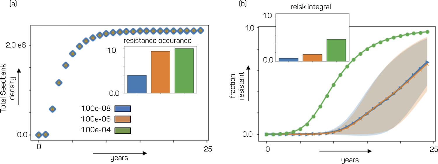
Several examples for the fraction of resistance are provided in Figure 5. For this example, the model is first run assuming different initial fraction of plants that are resistant (e.g., 1 plant in 1x10⁸ m²) to the herbicide. This is a sensitive parameter that often is not or cannot be easily measured and is often approximated. The relative percentage of simulations that do lead to resistance is given by the bar chart inset labeled resistance occurrence seen in Figure 5. The latent period is defined as the time (years) before any resistance is seen. Figures 6–12 follow the same format as Figure 5 (a) that represents the total seed back density over the entire number of the years simulated (e.g., 25 yrs.) while (b) represents the fraction of seeds where resistance is found. The fraction of resistance occurrence and the risk integral are provided by the bar chart insets. In several of the simulations, the predicted fraction of resistance seeds dies out (i.e., no resistance set in). Also, the variance is much less at that scale with such high allele frequency.

Figure 5
Example representing total seedbank density (a) and the fraction of resistant seed development over time (b) for three different initial allele resistance criteria (1.0e-08–1.0e-04)

3.2 Prediction Results with New Herbicide

Several analog experimental herbicides being considered for future product concepts in weed control are used here as examples for the modeling. The initial resistant frequency for Herbicide 1 was take as 1.0 × 10^-4(some resistance) and the resistant frequency for the other similar MOA Herbicide 2 was 1.0 ×10^-8 (little/no resistance). Mixing both herbicides helps keep the total weed density low. Using only Herbicide 1 increases the RI and using only herbicide 2 reduces resistance but at the cost of increased weed density seen in Figure 6.

Figure 6
Mixture of two discovery (e.g., not yet marketed) herbicides. (a) total seedbank density, (b) represents the fraction of resistance among the total population. Using only herbicide 2 will cause no resistance to build up on herbicide 1, which will result in an overall less resistance but at the cost of greater weed population

The relative number of times the weed sustains, or resistance occurs, is expressed in bar plot. Observations for the degree of sensitivity of the modelling pipeline to several input parameters, namely Initial seedbank density, Initial resistant allele frequency, and herbicide combinations is provided. Simulation examples for several similar (but not yet marketed) MoA herbicides are seen in Figure 6.

The total seedbank density per unit area is plotted for both resistant and non-resistant weed species (combined) for cases where the weed species don’t totally die out (e.g., extinction did not occur). The small standard deviation is not observed since the scale of the y axis is quite large. Thus, Figure 6 (a) expresses how the seedbank grows over time for both resistant and susceptible species for the number of cases where weeds are sustained. Figure 6 ((a), inset) is a bar chart representing the fraction of time among the 1,000 runs where the weeds developed resistant (if resistance did not develop, then the weed became extinct). The fraction of the weeds that are resistant to the herbicide is plotted only for cases where resistance set in as illustrated in Figure 6 (b).

Thus, the two graphics of Figure 6 represent only the cases with undesirable occurrence – for Figure 6 (a) weed growth and Figure 6 (b) resistance set in; where both the inset tell chances of weed sustenance or resistance risk overall. In Figure 6 it is observed that, with usage of combined herbicide, the weed density was less in the initial years followed by similar density in later years depicting the advantage of a combined herbicide application approach. As the resistant seedbank to herbicide 2 was smaller, fraction of times the resistance occurred was less (inset). The risk integral was lower for the cases where the initial seedbank was low, but with combined usage, the risk integral is like applying herbicide 1 alone. Analogous figures for different management practices are found in Figures 7–13.

3.3 Sensitivity Analysis

The effect of the initial seed bank density and initial frequency are shown in Table 2. Ideally, to minimize RI, this table provides a quick sensitivity analysis for the initial seed density and resistant allele frequency when two different herbicides are simulated (same MoA). Resistance thresholds for RO, CR, and TR are defined as 0.05, 0.30, and 0.95, respectively. Both resistance levels and overall future application rates for weed control were approximated via “best” guess approximations.

Table 2
Simulation results for several initial seed density and resistant allele frequencies impact on RO, CR, TR (time units are in years), and RI

Initial density	Initial frequency	RO time	CR time	TR time	RI
100	10-8	6.0	7.1	14.4	0.07
100	10-6	4.1	5.1	11.4	0.18
100	10-4	2.1	3.2	8.3	0.42
10	10-8	6.0	6.9	12.7	0.08
1,000	10-8	6.2	7.6	16	0.06

3.4 Initial Allele Frequency

Investigations into how the model reacts when assuming different initial allele frequencies (e.g., 1.0 x 10^-8 - 1.0 x 10^-4) is provided. As this frequency is increased, resistance occurrence also increases (Figure 7 (a)). This can be seen when plotting fraction resistant weeds (Figure 7 (b)) as resistance sets in earlier when the allele frequency is high.

Figure 7
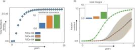
Effect of initial allele frequency. (a) total seedbank density, (b) represents the fraction of resistance among the total population

The seedbank frequency of resistant allele does not dramatically affect the total seedbank density. The seedbank frequency has been impacted via number of times resistance occur, and the Risk integral (RI) is higher with more resistant seedbank.

3.5 Seedbank Density

The effect of initial seed bank density is seen in Figure 8. Observations for seedbank density include small differences in the weed emergence during the initial phase, but during the later phase the density is similar, or the lower density catches up. Seedbank density influences the number of times resistance occurs, because lower density wipes out with higher probability by extinction event due to herbicide or natural causes. Resistance sets in quickly in lower density, as there is less competition from susceptible species. There is still probability that resistance would quickly set in for the case of lower density since this is a stochastic model (which also accounts for external factors). One of the external factors is intra and extra competition which is a stochastic quantity. This variable dominates the simulation outcome when the seedbank density is low.

Figure 8
Effect of initial seed bank density. (a) total seedbank density, (b) represents the fraction of resistance among the total population. Blue, orange, and green represent number of seeds per square meter

3.6 Herbicide Combination

Another plausible scenario is that significant resistance to the first herbicide has developed, and a second herbicide is introduced seen in Figure 9. Suppose that the initial frequency for gene locus 1 is 10^-4, and for gene locus 2 is 10^-8. The median RO, CR, and TR times are 6.1, 8.5, 11.4, and the average RI is 0.81, Table 3.

Figure 9
Treating a heavily resistant field with a second MOA. (a) total seedbank density, (b) represents the fraction of resistance among the total population

Table 3
Simulation results for two modes of action herbicides, where resistance has already been established for the first herbicide (initial resistant allele frequency 10-4) but not for the 2nd herbicide (initial resistant allele frequency 10-8). Units of time are in years

	RO time	CR time	TR time	RI
Herbicide 1 only	2.1	3.2	8.3	0.49
Herbicide 2 only	6.0	7.0	14.4	0.18
Herbicide 1 & 2	6.1	8.5	11.4	0.51

The initial condition is a variable fraction of resistance to begin with. Initial conditions for the first locus are 1.0×10^-4 and second locus is 1.0×10^-8. Now if one uses herbicide targeting each of the locus individually, between green indicating combined case and blue and orange pair considering individual case. Now if one uses herbicide 2 only, the risk integral will be smaller as indicated in the right figure because the Gene loci 1 will not offer resistance at all! But for the other two cases, as the starting frequency of gene loci 1 is higher, it imparts greater resistance if Herbicide 1 is used no matter what combined or individual cases are. The summary of this test is, in case two loci offers resistance, the fraction of resistance will be dominated by the one with more allele frequency. It is better to use a mixed herbicide having two different modes of action, and the model can capture what happens when one uses single mode vs mixed herbicide. For example, if one uses conceptualized 2 distinct herbicides acting on different alleles, then the difference seen between herbicide 1 and 2 is due to their characteristics, as they are distinctly different having their own set of parameters. The main takeaway from Figure 9 suggests what happens when mixed herbicides are used and what happens when one uses only one herbicide and ignores the other. Herbicide 2 is just another herbicide which works on different allele and having different/distinct property than herbicide 1.

Best option is using two MOA herbicides simultaneously as given by lower Risk Integral (RI) because although using single MoA with herbicide 2 indicated by orange line appears to have less fraction resistant in the right figure (Figure 9 (b)), the total seedbank density of weed is much higher as indicated in the left figure (Figure 9 (a)).

Mixing several herbicides together at application can keep the total weed density low. For this analysis, the resistant frequency for Herbicide 1 was 1.0 ×10^-4 and Herbicide 2 were 1.0 ×10^-8. One finds that when using only Herbicide 1 and/or a mixture increases the fraction resistant and risk integral. Using only Herbicide 2 reduces resistance but at the cost of increased weed density. For cases where two loci offer resistance, the fraction of resistance will be dominated by the one with more allele frequency.

3.7 Seed Delay

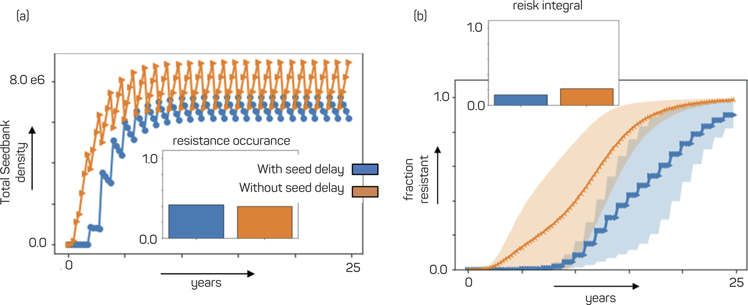
Table 4 provides simulation results when 4 weed cohorts are considered throughout the growing season with and without seed delay. Figure 10 (a) provides total seedbank density (includes both resistant and non-resistant seed. The relative percentage when resistance is manifest during the iterations is given by the internal graphic. Figure 10 (b) represents the fraction of resistance among the total population. Only cases where resistance is found are separated with the standard deviation plotted with the predictions. The area under the curve, once integrated, provides the Risk Integral (RI). The germination of the herbicide resistant seed with delay results in a step/saw-tooth like pattern.

Table 4
Simulation results for four cohorts with and without seed delay

	RO time	CR time	TR time	RI
four cohorts + seed delay	6.8	8.0	23.8	0.18
four cohorts no seed delay	1.5	1.9	10	0.24

Figure 10
A simulation with four cohorts illustrating the effect of seed delay. The winter survival fraction has been set to 0. (a) total seedbank density (includes both resistant and non-resistant seed, (b) represents the fraction of resistance among the total population

3.8 Management Strategies

Default settings are used to examine the effect of various management practices, Table 5. f_survival is the proportionality constant used in the survival expression. The default initial seed density and resistant allele frequencies for each herbicide are 100 sd/m² and 10^-8, respectively. These default values are set to both the upper and lower seed banks. Simulations for cultivation, hand weeding, and cover crops are carried out for OFF every year, ON and OFF in alternating years, and ON in all years. The effect of covering crops is to delay resistance as well, but its effect is even less pronounced than for cultivation and hand weeding.

Table 5
Default weed management configuration

Practice	Usage	Parameters
Cultivation	OFF	$f_{\text{surivol}}=\{\begin{array}{c}10FF\\ 0.050\mathrm{ON}\end{array}$
Hand weeding	OFF	$f_{\text{surivol}}=\{\begin{array}{c}10FF\\ 0.050\mathrm{ON}\end{array}$
Cover crop	OFF	$C=\{\begin{array}{c}0OFF\\ 5ON\end{array}$

3.9 Cultivation

The effect of cultivation is shown in Figure 11 with results summarized in Table 6. Resistance is delayed if cultivation is assumed (e.g., On) every year (and the risk integral is reduced). If there is cultivation each year, the seedbank density, or the number of weed per area will be considerably low in the initial year, with lower chance of occurring resistance [Figure 11 (a) and inset]. The risk integral is low with all year cultivation (Figure 11 inset). However, it appears resistance occurs faster (green line on top) then either alternate or no cultivation cases, which means once resistance has set in even after cultivation, then the fraction of resistant species will be much higher than the susceptible species which thrive after surviving cultivation, although that chance is low as RI is low (Figure 11 (b) inset). Thus, for the rare cases where resistance set in with cultivation (as per risk integral and resistance occurrence in Figure 11 (a) and (b) insets), the resistant plants get leverage as the competitor susceptible species gets eradicated and resistant fraction is higher early on.

Figure 11
Impact of cultivation on resistance increases over time. (a) total seedbank density, (b) represents the fraction of resistance among the total population. Cultivation for 3 cases: OFF all years, ON odd years + OFF even years, ON all years. Resistance is delayed most by always using cultivation

Table 6
Effect of cultivation on weed resistance impact. Cultivation what either fully On or Off or alternative On/Off over a 25 year simulation interval

	Off	On/Off	On
Median resistance onset time (years)	5.93 (45%)	8.79 (42%)	12.1 (26%)
Median critical resistance time (years)	7.64 (45%)	11.5 (42%)	20.0 (26%)
Median total resistance time (years)	9.77 (45%)	14.3 (42%)	24.2 (24%)
Average risk integral	0.37	0.30	0.15

3.10 Tilling

Finally, the effect of tilling is examined (Figure 12). Tillage turns soil over, so the upper seed bank becomes the lower, and visa versa. If seeds in the lower seed bank are more rapidly degraded, then this concept would always “work” but degradation of seeds in soil is slow and the reason why tillage predominantly only works once when implemented. Three cases are considered: No tilling, tilling at year 10, and tilling at year 10 and year 20, Table 7. In all cases, degradation in the lower seed bank is set to zero. One finds all three cases track together until year 10. As the no till case continues to rise with resistance, both tillage cases drop to nearly zero. The year 10 till case steadily increases, eventually reaching total resistance at around year 17. The year 20 till case suddenly jumps because there is no seed degradation in the lower seed bank. The highly resistant seeds which were buried at year 10 are reintroduced at year 20. Thus, depending on soil degradation conditions, more than one tillage may not decrease resistance. General Observations: 1 tillage over the product lifespan (25 years in this example) is the most sensitive management practice and any further tillage in subsequent years provided a diminishing return in terms of minimizing RI.

Figure 12
Impact of 0, 1, and 2 tillage events. (a) total seedbank density, (b) represents the fraction of resistance among the total population

Table 7
Effect of Tilling

	No Till	Till (year 10)	Till (Year 10 and Year 20)
Median resistance onset time (years)	5.93 (45%)	7.64 (72%)	13.7 (75%)
Median critical resistance time (years)	7.64 (45%)	16.5 (66%)	15.8 (56%)
Median total resistance time (years)	9.77 (45%)	26.9 (48%)	19.7 (50%)
Average risk integral	0.37	0.30	0.29

Possible extensions to this model include adding dormant periods for seeds within the seed bank before a seed germinates, and investigations into different number of chromosomes sets (e.g., polyploidy, where cells of a weed have more than one pair of chromosomes) acting upon several different places.

4.Conclusions

This model incorporates the impact of management practices on weed resistance that include cultivation, hand weeding, cover crop, herbicide application rates, and tillage. Tillage is one of the most sensitive management practices in reducing the onset of weed resistance. However, tillage effectiveness significantly diminishing after the first tillage event. Often it is desirable for the herbicide manufacture to manage a pesticide over the longevity of the product concept to maximize the profitability. If weed resistance within a field is greater than what a farmer deems acceptable, then the product concept has ended for this field as this specific herbicide will no longer be viable. An optimization approach can be used to showcase the novel ability to select Best Management Practices (BMPs) in such a way to maximize the profitability of the product over its lifetime and minimize the onset of resistance. Once resistance within a field increases above a critical level that farmers notice (and crop yields are reduced), then this acreage can no longer contribute to the profitably in subsequent years.

The mechanics of this model, as outlined in this paper, was then used to simulate the future behavior of several new molecules in an industrial company’s discovery process. In this way, predictive onset of resistance and the best ways to manage the predevelopment herbicide in moving forward can be considered. Sensitive model inputs are also found to provide a mechanism to refine model predictions as these parameters require the best measured values since small changes in these parameters create the greatest variance in output. This tool can help chemical manufacturers prioritize lead molecules in their discovery process (should multiple compounds be in the pipeline), but only limited resources are available, etc. Development of this tool is a first step in addressing potential resistance issues in the future and provides a starting platform for future expansion and modifications as refined experimental information regarding sensitive model inputs becomes available. A final note not covered here is the use of novel AI techniques to process vast amounts of data and uncover intricate patterns for predicting and managing herbicide resistance in a more precise and proactive manner (Ghatrehsamani et al., 2023). This tool, and others like it, can be used to prioritize early development molecules in the manufactures pipeline.

Figure 2
Original Pipeline where multiple transfer functions take a population, perform and operation, and return a new population (West et al., 2018)

Acknowledgements

We thank Corteva employees Jeremy Kister and Norbert Satchivi who provided information for several experimental herbicides simulated herein and Corteva managers Navin Elango and David Mann, along with colleagues Hudson Takano, Mamadou Kane Mboup, Paul Schmitzer, Amit Sethi, and Lucas Bobadilla for feedback and future directions to consider.

References

• Bagavathiannan M, Norsworthy, J. Modeling the evolution of herbicide resistance in weeds: current knowledge and future directions. Ind J Weed Sci. 2016;48(2):122-7. Available from: https://doi.org/10.5958/0974-8164.2016.00032.0
  » https://doi.org/10.5958/0974-8164.2016.00032.0
• Gerhards R, Sanchez DA, Hamouz P, Peteinatos GG, Christensen S, Fernandez-Quintanilla C. Advances in site-specific weed management in agriculture: a review. Weed Res. Weed Res, 2022,62(2)123-133. Available from: https://doi.org/10.1111/wre.12526
  » https://doi.org/10.1111/wre.12526
• Ghatrehsamani S, Jha G, Dutta W, Molaei F, Nazrul F, Fortin M et al. Artificial intelligence tools and techniques to combat herbicide resistant weeds: a review. Sustainability. 2023;15(3):1-18. Available from: https://doi.org/10.3390/su15031843
  » https://doi.org/10.3390/su15031843
• Heap I. The international survey of herbicide resistant weeds. Weedscience. 2023[access Sept 1, 2023]. Available from: www.weedscience.org
  » www.weedscience.org
• Holmes KH, Lindquist JL, Rebarber R, Werle R, Yerka M, Tenhumberg B. Modeling the evolution of herbicide resistance in weed species with a complex life cycle. Ecol Applic. 2022;32(1):1-19. Available from: https://doi.org/10.1002/eap.2473
  » https://doi.org/10.1002/eap.2473
• Lauenroth D, Gokhale CS. Theoretical assessment of persistence and adaptation in weeds with complex life cycles. Nat Plants. 2023;9:1267-79. Available from: https://doi.org/10.1038/s41477-023-01482-1
  » https://doi.org/10.1038/s41477-023-01482-1
• Liu C, Jackson LV, Hutchings SJ, Tuesca D, Moreno R, Mcindoe E et a l. A holistic approach in herbicide resistance research and management: from resistance detection to sustainable weed control. Scient Rep. 2020;10:1-9. Available from: https://doi.org/10.1038/s41598-020-77649-z
  » https://doi.org/10.1038/s41598-020-77649-z
• Maxwell BD, Roush ML, Radosevich SR. Prediction the evolution and dynamics of herbicide resistance in weed populations. Weed Technol. 1990;4(1):2-13. Available from: https://doi.org/10.1017/S0890037X0002488X
  » https://doi.org/10.1017/S0890037X0002488X
• Mayo O. A century of hardy-weinberg equilibrium. Twin Res Human Gen. 2008;11(3):249-56. Available from: https://doi.org/10.1375/twin.11.3.249
  » https://doi.org/10.1375/twin.11.3.249
• Neve P, Norsworthy JK, Smith KL, Zelaya IA. Modelling evolution and management of glyphosate resistance in Amaranthus palmeri. Weed Res. 2011a;51(2):99-112. Available from: https://doi.org/10.1111/j.1365-3180.2010.00838.x
  » https://doi.org/10.1111/j.1365-3180.2010.00838.x
• Neve P, Norsworthy JK, Smith KL, Zelaya IA. Modeling glyphosate resistance management strategies for Palmer amaranth ( Amaranthus palmeri ) in cotton. Weed Technol. 2011b;25(3):335-43. Available from: https://doi.org/10.1614/WT-D-10-00171.1
  » https://doi.org/10.1614/WT-D-10-00171.1
• Sack H. G. H. Hardy and the aesthetics of mathematics. SciHi Blog. December 1, 2022.
• Somerville GJ, Powles SB, Walsh JJ, Renton M. How do spatial heterogeneity and dispersal in weed population models affect predictions of herbicide resistance evolution? Ecol Modell. 2017;362:37-53. Available from: https://doi.org/10.1016/j.ecolmodel.2017.08.002
  » https://doi.org/10.1016/j.ecolmodel.2017.08.002
• Weinberg W. [On the proof of inheritance in humans]. Jahreshefte des Vereins für Vaterländische Naturkunde in Württemberg. 1908. German.
• West A, Altieri A, Cryer SA. Generalized management strategies to delay herbicide resistance: a simulation approach. Weed Sci. 2018;66(4):530-9. Available from: https://doi.org/10.1017/wsc.2018.13
  » https://doi.org/10.1017/wsc.2018.13

• Funding:
  This research was fully funded by Corteva Agriscience and received no external funding.

Edited by

• Editor in Chief:
  Carol Ann Mallory-Smith

• Associate Editor:
  Anderson Luis Nunes

Publication Dates

• Publication in this collection
  22 Nov 2024
• Date of issue
  2024

History

• Received
  19 Apr 2024
• Accepted
  18 Sept 2024