
 Does a computational routine help in the assertive definition of herbicide doses for isobologram analysis?
Abstract:
Weeds are a problem for the development of agricultural crops, mainly due to the acquired resistance to herbicides. One approach to weed control is based on the chemical method, using herbicides in a mixture. However, herbicide combinations are complex and may lead to synergistic, antagonistic, or additive effects. One way of evaluating this effect is by means of isobolograms, the doses of which have previously been defined using dose response curve studies. The determination of doses for isobologram construction can be based on the relative potency of the ED50 values, defined as the ratio between the doses of the two herbicides that produce a 50% effect. Nevertheless, calculating these doses manually or using spreadsheets carries a risk of operational errors, potentially leading to incorrect decisions. The aim of this study was to present a computational routine in the R software to help define doses for isobologram studies. To do this, data from four dose-response curve experiments conducted in a completely randomized design under greenhouse conditions were used to obtain the necessary doses. In the same time, doses obtained using Microsoft Excel to validate the proposed methodology. The same results were obtained using the spreadsheet and the proposed routine, but in R it was with more agility, practicality and with the work centralized in the same software.
Keywords:
Dose-response curve; relative potency; herbicide mixture; automation in R; Euphorbia heterophylla; Amaranthus hybridus
1. Introduction
Weeds interfere with the growth and development of agricultural crops by competing for essential resources such as water, light, nutrients, and space (Vasconcelos, Silva, and Lima, 2012). In order to avoid the negative interference from weeds, various control methods should be adopted, with emphasis on chemical control. Herbicides account for 67% of all pesticides used globally, highlighting the widespread adoption of this approach across more than 4,78 billion hectares of arable land worldwide (FAO, 2024). However, one of the limitations of chemical control is the emergence of herbicide resistant weed species, with 534 cases currently reported worldwide, with 21 involving resistance to modes of action and 168 to specific herbicides (HEAP, 2025).
Worldwide, there are 1526 known cases of herbicide resistance in more than 200 weeds species. Of these, 40% involve resistance to acetolactate synthase (ALS) inhibitors, 24% to 5-enolpyruvyl shikimate-3-phosphate synthase (EPSPs) inhibitors, and 22% to photosystem II (PS II) inhibitors. These cases include instances of single, multiple, or cross-resistance (HEAP, 2025). Cases of resistance to EPSPs inhibitors are important for soybean cultivation, given that worldwide this crop covers more than 75 million hectares (FAO, 2025). Brazil is the largest producer of this oilseed, due to the widespread adoption of tolerance technology to the herbicide glyphosate, which is present in 95% of the more than 46 million hectares under soybean cultivated in Brazil (Henning and Nepomuceno, 2022; CONAB, 2024).
Among the glyphosate resistant weed species in Brazil, wild poinsettia (Euphorbia heterophylla L.) and smooth pigweed (Amaranthus hybridus L.) stand out, with resistance reported in 2019 and 2018, respectively (HEAP, 2025). In addition to glyphosate resistance, E. heterophylla also shows resistance to ALS inhibiting herbicides and protoporphyrinogen oxidase (PPO) inhibitors (Trezzi et al., 2005; Grazziero et al., 1998). A. hybridus, in turn, exhibits multiple resistance to both EPSPs and ALS inhibitors (Oliveira et al., 2024).
Given this scenario, the use of herbicides in a mixture becomes important, being an alternative adopted by 90% of producers to manage resistance in pre-seeding soybean (Ulguim et al., 2017). Accordingly, to another study found that approximately 97% of producers use pesticide mixtures, in soybean production specifically, glyphosate is mixed in 86% of applications with other pesticides, indicating a strategy to extend control and manage resistance (Grazziero et al., 2015). By combining herbicides with different modes of action, the chance of the weed developing resistance is not only reduced, but also delayed, increasing the chances of control. The mixture can result in synergistic, antagonistic, or additive interactions, due to physicochemical reactions or physiological changes that occur in the plant after herbicide absorption (Barbieri et al., 2022). For a synergistic effect to occur, the mixture should provide greater control than that expected from herbicides applied individually (Avila-Neto et al., 2024). One way to evaluate these interactions is through the isobologram methodology.
The use of isobolograms originated in the field of pharmacology and was first applied to weed science by Tammes (1964), and it is commonly used in studies aimed at understanding the effects of herbicide mixtures (Avila-Neto et al., 2024; Mario et al., 2023). The isobologram involves combining herbicides in different proportions and doses. In the graphical representation, the ED50 values of each herbicide applied individually are connected by a line known as the line of additivity. Based on this line, the ED50 values of mixtures at different proportions are plotted on the graph. Depending on the position of these points relative to the additivity line, the interactions can be classified as synergistic, if the points are below the line; antagonistic if they are above it; or additive when the points are on the additivity line. This interpretation is carried out by considerating the confidence intervals of the estimated ED50 values, both for individual herbicides and for their mixtures (Kruse, Vidal, and Trezzi, 2006).
One of the important steps for the success of the methodology is the definition of relative potency, which consists of the ratio of effective doses that cause a certain level of response, such as ED50, for example. Relative potency can also be explained as the biological exchange rate, it indicates the proportion in which one herbicide can substitute another to achieve the same effect (Barbieri et al., 2022). Therefore, it is essential to assess the sensitivity of weed species to herbicides before initiating isobologram studies. One approach is to expose the target species to increasing herbicide doses using dose-response curves, and to estimate the ED50 of each herbicide before constructing the isobologram (Kalkhoran et al., 2021).
After determining the ED50 values for each herbicide individually, the next stage in constructing isobolograms involves calculating the mixture doses to be tested. This stage is time-consuming and susceptible to operational errors, especially when working with a large volume of data generated by herbicide combinations, and can be carried out using electronic spreadsheets such as Microsoft Excel, or even more arduously, manually.
Data analysis has been transformed by the rise of more accessible statistical software, such as R, developed in the 1990s by Ross Ihaka and Robert Gentleman (Ihaka and Gentleman, 1996). Its adoption has made it possible to give the researcher more autonomy, which, combined with the rise of the internet, has made scientific research more collaborative. As an open source language with a wide range of statistical packages, R has made data analysis faster and more accessible. Another important advance was the emergence of the RStudio software in 2010, which is an environment integrated with R that facilitates the execution, organization and resumption of codes, as well as being free and allowing the management of projects and directories with practicality (Battisti and Smolski, 2019).
In view of this, the use of R software (R Core Team, 2019) has emerged as an alternative to assist in research with isobolograms. Thus, the aim of this study was to propose a computational routine in R that automates the process of determining herbicide mixture doses at different proportions, facilitating the implementation of the isobologram methodology.
2. Material and Methods
2.1 Plant Material and Experimental Design
Dose-response curve experiments were carried out with Euphorbia heterophylla and Amaranthus hybridus, with each dose-response curve considered as a separate experiment. In total, four experiments were conducted, each replicated twice, in a greenhouse at the Department of Plant Protection of the Federal University of Santa Maria, between April and December 2024. The experimental design was completely randomized. The first experiments with E. heterophylla included four replications, and the second ones had three replications. The same design was applied to the Amaranthus hybridus experiments. The dose-response curves for both weed species were performed using the herbicides 2,4-D choline salt and thiafenacil. The experimental units for the E. heterophylla trials consisted of 0,3 L pots, while those for A. hybridus used 0,2 L pots, all filled with previously sieved soil. Soil fertility was corrected by applying 200 kg ha-1 of 05-20-20 fertilizer. The soil used in the experiments was classified as an ultisol (Pes and Arenhardt, 2015).
For the Euphorbia heterophylla experiments, seeds from a biotype with no recorded herbicide resistance were used, collected in Engenheiro Coelho – SP (22°30’25.7"S, 47°10’38.6"W). Seed dormancy was broken through mechanical scarification using sandpaper. Afterward, the seeds were placed in gerbox containers on germination paper moistened with distilled water at a ratio of 2,5 times the paper's weight. The containers were kept in growth chambers for 48 hours at 25°C with a 12-hour photoperiod. Newly germinated seeds were then transferred to cell trays containing soil, where they were grown until the four-leaf stage.
Uniform Euphorbia heterophylla seedlings were individually transplanted into pots with intact root clods. When the plants reached the two true-leaf stage, topdressing was applied at a rate of 200 kg ha-1 using the 45-0-0 fertilizer formulation.
For the Amaranthus hybridus experiments, seeds were sown in cell trays filled with soil, as previously described. Once the seedlings emerged and developed two cotyledonary leaves, they were transplanted into 0.2 L pots. Upon reaching the two true-leaf stage, they received topdressing with 200 kg ha-1 of the 45-0-0 (NPK) fertilizer.
2.2 Treataments and application
The treatment factor consisted of increasing doses of 2,4-D choline salt or thiafenacil applied individually (Table 1). Applications were carried out when Euphorbia heterophylla plants reached the four to five true leaf stage, while for Amaranthus hybridus the herbicides were applied when plants had four to six true leaves (first experimental replication) or six to eight true leaves (second replication).
Herbicide treatments applied to Euphorbia heterophylla and Amaranthus hybridus plants in relation to the commercial label rates of 2,4-D choline salt and thiafenacil, expressed in ml, g a.e. ha-1 or g a.i. ha-1. Santa Maria, 2024.
The treatments were applied using a CO2 pressurized backpack sprayer equipped with Airmix® 110.015 nozzles, calibrated to deliver a spray volume of 150 L ha-1. For the experiments with the herbicide thiafenacil, the adjuvant Lanzar® was added at 0,5% v/v of the spray solution, as recommended. After application, the plants were kept spaced apart in a well-ventilated, shaded environment for 8 hours before being returned to the greenhouse.
2.3 Variables evaluated and data analysis
The variable evaluated was the dry mass of the aerial part (DM) at 21 days after application (DAA) for Euphorbia heterophylla and 28 DAA for Amaranthus hybridus. Plants were cut at the base, close to the soil surface, and the plant material was stored in paper bags and dried in an oven for 72 hours or until a constant weight was achieved at 60°C. Afterwards, the samples were weighed on a precision scale, and the data were expressed in grams per plant (g plant-1).
Data were tested for adherence to assumptions using R software (R CORE TEAM, 2019), and the four-parameter log-logistic model (Equation 1) was fitted using the drc package (Ritz et al., 2015). A significant level of 0,05 was adopted for all statistical analyses.
where: y = variable analyzed; b = slope of the curve; c = lower limit of the regression; d = upper limit of the regression; x = herbicide dose; ED50 = the dose that causes a 50% reduction in dry mass.
The verification of the model assumptions was carried out using the Shapiro-Wilk, Bartlett, and Durbin-Watson tests, respectively for normality, homogeneity, and independence of errors. In addition to that verification, lack of fit was tested (Ritz et al., 2015) and the confidence interval was obtained via bootstrap resampling (Efron, 1979), adopted to obtain model parameters in the analysis of variance that violated any of the assumptions.
To analyze the data using the proposed computational routine, the Excel spreadsheet must be structured as shown in Table 2. The number of treatments, replicates, and the use of blocks (or not) is entirely at the researcher's discretion.
Basic data structure in Excel format to be loaded into the computational routine for obtaining the doses for the isobologram.
2.4 Development of the computational routine in R
The choice of names for the objects created in R is up to the researcher, however, each object is referred to using the terms presented in Table 3. All intrinsic R functions and package-specific commands used in the routine are summarized in Table 4. To analyze the data from the experiments, the packages were used and loaded according to the script:
-
require(MASS)
-
require(ExpDes.pt)
-
require(ggplot2)
-
require(dplyr)
-
require(agricolae)
-
require(pastecs)
-
require(xlsx)
-
require(car)
-
require(boot)
R functions/commands and packages used in the computational routine (fixed names, not alterable).
Afterwards, the data from the dose–response curve experiment of the first herbicide, 2,4-D choline salt, referred to as "HerbicideA", was uploaded. Analysis of variance (Anova) was then performed, along with an assessment of the assumptions for the variable DM, named "Drymass".
attach(HerbicideA)
AnovaHerbicideA <- dic(Treat, Drymass, quali = FALSE)
Dic_model <- lm(Drymass~ as.factor(Treat), data = HerbicideA)
durbinWatsonTest(Dic_model)
The four-parameter model was then estimated. To accomplish this, the drc package (Ritz et al., 2015) was loaded, and the attach function was used to make the dataset available in the search path.
Drymass_A <- drm(Drymass ~ dose, data = HerbicideA, fct = LL.4())
The summary function generates a statistical summary of the object passed as an argument. The modelFit function is used to evaluate the fit of non-linear models applied to dose-response curves, and the ed_values function calculates the dose that produces a given level of response, in this case, 50. To obtain a satisfactory model fit, the p-value must be greater than or equal to 0,05.
summary(Drymass_A)
modelFit(Drymass_A)
ed_values_A <- ED(Drymass_A, c(50), interval = "delta")
Bootstrap resampling analysis was used to generate 95% confidence intervals (95% CI). The get_params function fits the model to each subsample and returns the four estimated parameters. The try function prevents the process from failing by returning NA when the model cannot be fitted. The set.seed(123) function ensures reproducibility. The boot function performs the desired number of resamplings, in this case, 1000, and boot.ci computes the confidence intervals for the parameters. The colMeans function calculates the mean of the values obtained from the bootstrap resampling, which is used as the final estimate for parameters b, c, d, and e.
get_params <- function(data, indices) {
d <- data[indices, ]
fit <- try(drm(Drymass ~ dose, data = d, fct = LL.4()), silent = TRUE)
if (inherits(fit, "try-error")) rep(NA, 4) else coef(fit)}
set.seed(123)
boot_results <- boot(data = HerbicideA, statistic = get_params, R = 1000)
for (i in 1:4) print(boot.ci(boot_results, type = "perc", index = i))
params_mean_A <- setNames(colMeans(boot_results$t, na.rm = TRUE), c("b", "c", "d", "e"))
print(params_mean_A)
After carrying out the analysis for the first herbicide (HerbicideA, corresponding to 2,4-D choline salt), the same process was applied to the second herbicide (HerbicideB), in this case thiafenacil, based on the same script:
attach(HerbicideB)
AnovaHerbicideB <- dic(Treat, Drymass, quali = FALSE)
Dic_model <- lm(Drymass ~ as.factor(Treat), data = HerbicideB)
durbinWatsonTest(Dic_model)
Drymass_B <- drm(Drymass ~ dose, data = HerbicideB, fct = LL.4())
summary(Drymass_B)
modelFit(Drymass_B)
ed_values_B <- ED(Drymass_B, c(50), interval = "delta")
get_params <- function(data, indices) {
d <- data[indices, ]
fit <- try(drm(Drymass ~ dose, data = d, fct = LL.4()), silent = TRUE)
if (inherits(fit, "try-error")) rep(NA, 4) else coef(fit)}
set.seed(123)
boot_results <- boot(data = HerbicideB, statistic = get_params, R = 1000)
for (i in 1:4) print(boot.ci(boot_results, type = "perc", index = i))
params_mean_B <- setNames(colMeans(boot_results$t, na.rm = TRUE), c("b", "c", "d", "e"))
print(params_mean_B)
For the experiments without violation of assumptions, the ED50 of the herbicides was extracted, the relative potency was calculated and its value was displayed according to the following command:
ED50_A <- ed_values_A[1]
ED50_B <- ed_values_B[1]
relative_potency <- ED50_A / ED50_B
print(relative_potency)
For the experiments that did not meet any of the assumptions, the parameters obtained through bootstrap resampling were used. To do this, objects with different names were created to calculate the relative potency in these cases:
ED50_bootstrap_A <- params_mean_A["e"]
ED50_bootstrap_B <- params_mean_B["e"]
relative_potency_boot <- ED50_bootstrap_A / ED50_bootstrap_B
print(relative_potency_boot)
To calculate the relative potency, the equation proposed by Ritz et al. (2015) was adapted, as shown below:
ZA e ZB are the doses of each herbicide applied individually that cause a specific effect, as used by the authors, in this case, a 50% response. This equation was adapted to be displayed in the "Source" field. With this parameter obtained, the doses to be used in the isobologram were calculated using Equation 3, proposed by Finney (1971).
where Za and Zb are the doses of each herbicide applied alone, and za and zb are the doses in mixture. This equation defines a line of additivity, which serves as a reference to detect possible synergistic or antagonistic interactions. By substituting the relative potency ratio into Equation 3, Equation 4 is obtained, adapted from Streibig and Jensen (2000):
This equation was adapted for direct calculation in R. Subsequently, the mixture doses of each herbicide were obtained for each proportion using the equation above, with the following command:
proportions <- data.frame(A = c(100, 75, 50, 25, 0), B = c(0, 25, 50, 75, 100))
proportions$za <- (proportions$A / 100) * ED50_bootstrap_A # or use ED50_A
proportions$zb <- (1 - (proportions$za / ED50_bootstrap_A)) * ED50_bootstrap_B # or use ED50_B
In this way, a "data frame" was generated where it is possible to combine different proportions of herbicide mixture doses. See below:
-
doses <- data.frame()
-
for (i in 1:nrow(proportions)) {
-
za_central <- proportions$za[i]
-
zb_central <- proportions$zb[i]
With the data frame created, the next step was to add the doses of interest to be tested. The previously calculated ED50 values of the herbicides were used as a reference, considering 9 doses in total, 4 above and 4 below the ED50. Therefore:
za_doses <- za_central * c(0, 1/16, 1/8, 1/4, 1/2, 1, 2, 4, 8)
zb_doses <- zb_central * c(0, 1/16, 1/8, 1/4, 1/2, 1, 2, 4, 8)
Afterwards, a temporary data frame with the combined doses was created and added to the main data frame:
temp_df <- data.frame(
Proportion = paste(proportions$A[i], ":", proportions$B[i], sep = ""),
za = za_doses,
zb = zb_doses )
doses <- rbind(doses, temp_df) }
Finally, the print function displays in the Console a table called "doses" that was generated above.
print(doses)
The complete computational routine is presented in Table 5. The choice of doses is at the researcher's discretion and should be adjusted as needed, since the successful continuation of the computational routine without errors depends on this.
2.5 Obtaining mixture doses using Microsoft Excel
One of the ways of calculating doses is through electronic spreadsheets, using Microsoft Excel. To validate the computer routine, the procedure for obtaining doses using Microsoft Excel was carried out. To do this, it was necessary to create a table with the ED50 of each herbicide, another table with the doses above and below those generated by ADM, using equations 1, 2 and 3, and finally, another table with the final result, as shown in the flowchart (Figure 1).
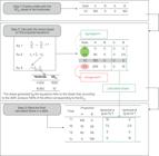
Flowchart of the step-by-step procedure using Microsoft Excel to generate the doses composing the isobologram, in order to validate the computational routine proposed in this study.
3. Results and Discussion
The data obtained for the DM variable fit the four-parameter log-logistic model for both herbicides in the second experiment with 2,4-D choline salt and in the second experiment with thiafenacil on Euphorbia heterophylla, as well as for the first and second experiments with 2,4-D choline salt on Amaranthus hybridus.
The first experiments with 2,4-D choline salt and thiafenacil on Euphorbia heterophylla, as well as the first and second experiments with thiafenacil on Amaranthus hybridus, did not meet some of the assumptions. The verification of Anova assumptions indicated that the residuals followed a normal distribution (Shapiro-Wilk test, p ≥ 0,05), showed homogeneity of variances (Bartlett test, p ≥ 0,05), and exhibited no correlation (Durbin-Watson test, p ≥ 0,05) across all experiments. Exceptions were noted for the Shapiro-Wilk test in the first experiment with thiafenacil on E. heterophylla, and for the Bartlett test in the first experiment with 2,4-D choline salt on E. heterophylla, the first experiment with thiafenacil on E. heterophylla, and the first experiment with thiafenacil on A. hybridus. The lack-of-fit test indicated that the four-parameter model was adequate to describe the dose-response relationship for the herbicide 2,4-D choline salt in all experiments, except for the second experiment with thiafenacil on A. hybridus (p ≥ 0,05). For the experiments that did not meet some of the assumptions of the analysis of variance or the nonlinear model, parameters were obtained via bootstrap resampling.
The ED50 values indicate that the herbicide thiafenacil, both for Euphorbia heterophylla and Amaranthus hybridus, showed greater efficiency in reducing DM compared to 2,4-D choline salt, requiring a smaller amount in grams of active ingredient (acid equivalent for 2,4-D choline salt) to reduce DM (Table 6). This indicates that thiafenacil can achieve a 50% reduction in DM of these plants with low doses (< 7 g a.i. ha–1).
Four-parameter log-logistic model estimates or bootstrap resampling for the first (1) and second (2) replication of the dose-response curve experiment with the herbicides 2,4-D choline salt and thiafenacil conducted in a greenhouse for Euphorbia heterophylla and Amaranthus hybridus. Santa Maria, 2024.
For the experiments with Euphorbia heterophylla, the "e" parameter indicating the ED50 was 620,09 g and 426,95 g a.e. ha-1 for the herbicide 2,4-D choline salt, while for thiafenacil the estimated parameter was 6,88 g and 3,33 g a.i. ha-1 for the first and second repetitions of the experiments (Table 6), respectively. These estimated parameters generated a relative potency of 90,14 and 128,17. For the experiments with Amaranthus hybridus, ED50 values of 46,54 g and 36,97 g a.e. ha-1 were found for 2,4-D choline salt and 0,87 g and 2,24 g a.i. ha-1 for thiafenacil for the first and second repetitions of the experiments, respectively, resulting in relative potencies of 53,49 and 16,50.
A reduction in relative potency was observed for the experiments with Amaranthus hybridus on plants with six to eight leaves. This occurred due to an increase in the ED50 parameter of the herbicide thiafenacil in the first repetition of the experiment with the same herbicide (from 0,87 to 2,24 g a.i. ha-1), or due to a decrease in this parameter for the herbicide 2,4-D choline salt (from 46,54 to 36,97 g a.e. ha−1).
The ED50 parameter from equations fitted to protox enzyme inhibition data by different herbicides in Amaranthus spp., Arabidopsis spp., Glycine max (L.) Merr., and Conyza spp. was three to nine times higher for oxifluorfen and fomesafen compared to thiafenacil (Park et al., 2018). This result is consistent with what was observed for Euphorbia heterophylla and Amaranthus hybridus, where the ED50 values were considered low for the DM variable (Table 6). In addition, it was observed that a dose of thiafenacil corresponding to 12 g a.i. ha-1 provided control of Echinochloa colonum (L.) Link. and Echinochloa crus-galli (L.) Beauv. above 95% (Laguerre et al., 2024), confirming the the effect of the herbicide at low doses.
The relative potency values observed in this study for Euphorbia heterophylla (90,14 and 128,17) indicate a low amount of the active ingredient thiafenacil (6,88 g a.i. ha-1 and 3,33 g a.i. ha-1) required to cause the same effect as a higher dose of 2,4-D choline salt (620,09 g a.e. ha-1 and 426,95 g a.e. ha-1). A relative potency of 71.32 for flumioxazin compared to metribuzin in potato (Solanum tuberosum L.) control was found (Kalkhoran et al., 2021), while another study reported ED50 values of 551,6 and 6,3 g a.i. ha-1 for propaquizafop and pinoxaden, respectively, for the reduction of DM in wild oats (Avena fatua), which corresponds to a relative potency of 87,55 (Vijayarajan et al., 2020), similar to that found in the relationship between the first experiments with 2,4-D choline salt and thiafenacil in E. heterophylla (90,14). ED50 values for 2,4-D amine and sulfosulfuron for DM reduction, ranging from 158,5 to 289,51 g a.i. ha-1 (131,79 to 240,84 g a.e. ha-1) and 2,73 to 5,64 g a.i. ha-1, respectively, were observed in a study under different water hardness conditions (Voojodi et al., 2023), which reported relative potency values between 42,70 and 48,27.
The calculation of relative potency was applied to generate the doses and mixture proportions presented in Table 7, which was adapted from the R output shown in Figure 2. The calculations were based on the relative potency obtained from the first experiments with Euphorbia heterophylla (90,14). The same results were obtained when performing the calculations manually in Microsoft Excel, although this method was more time-consuming. Furthermore, when working with the computational routine in R, it is possible to carry out all the steps within the same software, requiring only the input of the dose-response curve data files. When using spreadsheets to construct doses, must first be analyzed and assumptions checked using statistical software. Making it possible to analyze the dose response curve data and obtain the doses for the isobologram in the same software, and also in the same computer routine, makes the process faster and less costly.
Doses generated for the isobologram using the computational routine in R software based on the ED50 from the first and second experiments with Euphorbia heterophylla.

Screenshot of the R output environment showing the final result of the dose calculation to be used in the isobologram.
4. Conclusions
The computational routine developed in R was efficient for calculating the doses of 2,4-D choline salt and thiafenacil to be used in studies involving isobolograms studies. Automation makes the process of obtaining mixture doses more agile and simple, based on R programming, which reduces the likelihood of operational errors and centralizes the work within R. The study developed can support the initial part of obtaining data and researchers who study mixtures of herbicides with isobolograms.
Acknowledgements
The authors would like to thank the Herbology Group at UFSM for their help during the experiments.
References
-
Avila-Neto R, Ulguim AR, Schneider T, Fortuna C, Holkem AS, Somavilla IP. Interaction between saflufenacil and ammonium glufosinate to control ryegrass. Braz. J. Biol. 2024;84: e286456. Available from: https://doi.org/10.1590/1519-6984.286456
» https://doi.org/10.1590/1519-6984.286456 -
Barbieri GF, Young BG, Dayan FE, Streibig JC, Takano HK, Merotto Jr A, et al. Herbicide mixtures: interactions and modeling. Adv Weed Sci. 2022;40(1): e020220051. Available from: https://doi.org/10.51694/AdvWeedSci/2022;40:seventy-five011
» https://doi.org/10.51694/AdvWeedSci/2022;40:seventy-five011 - Battisti IDE, Smolski FMS. [R software: Statistical data analysis using a free program]. Bagé: Editora Faith; 2019. 173 p. Portuguese.
-
CONAB – Companhia Nacional de Abastecimento. [7th Survey – 2024/25 Harvest. Grain Crop Bulletin]. Portuguese. Available from: https://www.gov.br/conab/pt-br/atuacao/informacoes-agropecuarias/safras/safra-de-graos/boletim-da-safra-de-graos/7o-levantamento-safra-2024-25/7o-levantamento-safra-2024-25 Acessed: Apr 2025.
» https://www.gov.br/conab/pt-br/atuacao/informacoes-agropecuarias/safras/safra-de-graos/boletim-da-safra-de-graos/7o-levantamento-safra-2024-25/7o-levantamento-safra-2024-25 -
Efron B. Bootstrap Methods: Another Look at the Jackknife. Ann. Statist. 1979;7(1):1-26. Available from: https://doi.org/10.1214/aos/1176344552
» https://doi.org/10.1214/aos/1176344552 -
FAO. Land statistics 2001-2022. Global, regional and country trends. 2024. Available from: https://openknowledge.fao.org/items/6c17080e-6c5d-47ae-a982-609c882bd4e7
» https://openknowledge.fao.org/items/6c17080e-6c5d-47ae-a982-609c882bd4e7 -
Grazziero DLP, Brighenti AM, Maciel CDG, Christoffoleti PJ, Adegas FS, Voll E. [Resistance of wild poinsettia to herbicides that inhibit the ALS enzyme]. Planta Daninha. 1998;16(2):117–125. Portuguese. Available from: https://doi.org/10.1590/S0100-83581998000200005
» https://doi.org/10.1590/S0100-83581998000200005 -
Grazziero DLP. [Mixtures of pesticides in tank, in Brazilian farms]. Planta Daninha. 2015;33(1):83–92. Portuguese. Available from: https://doi.org/10.1590/S0100-83582015000100010
» https://doi.org/10.1590/S0100-83582015000100010 -
Heap, I. The International Herbicide-Resistant Weed Database. Online. Tuesday, April 22, 2025. Available from: http://www.weedscience.org/
» http://www.weedscience.org/ -
Henning FA, Nepomuceno AL. [Biotechnology in the development of soybean cultivars]. Seed News. Available from: https://seednews.com.br/artigos/4007-biotecnologia-no-desenvolvimento-de-cultivares-de-soja-edicao-setembro-2022 Portuguese. Accessed Apr 2025.
» https://seednews.com.br/artigos/4007-biotecnologia-no-desenvolvimento-de-cultivares-de-soja-edicao-setembro-2022 -
Ihaka R, Gentleman R. A Language for Data Analysis and Graphics. J. Comput. Graph. Stat. 1996;5(3):299–314. Available from: https://doi.org/10.1080/10618600.1996.10474713
» https://doi.org/10.1080/10618600.1996.10474713 -
Kalkhoran ES, Alebrahim MT, Abad HRMC, Streibig JC, Ghavidel A, Tseng TMP. The Joint Action of Some Broadleaf Herbicides on Potato (Solanum tuberosum L.) Weeds and Photosynthetic Performance of Potato. Agriculture. 2021;11(1103):1-17. Available from: https://doi.org/10.3390/agriculture11111103
» https://doi.org/10.3390/agriculture11111103 -
Kruse ND, Vidal RA, Trezzi MM. Dose-Response Curve and Isobologram Used to Describe the Mixture of Herbicides Inhibitors of the Photosystem II and Carotenoid Synthesis. Planta Daninha. 2006;24(3):579-587. Available from: https://doi.org/10.1590/S0100-83582006000300022
» https://doi.org/10.1590/S0100-83582006000300022 -
Laguerre G, Contreras Jr A, Hanson BD. Evaluation of weed control efficacy and crop safety of the PPO-inhibiting herbicide thiafenacil in California orchard cropping systems. Weed Technol. 2024;38(46):1-8. Available from: https://doi.org/10.1017/wet.2024.46
» https://doi.org/10.1017/wet.2024.46 -
Mario RB, Ulguim AR, Avila-Neto RC, Campos PV, Corrêa AR, Brandão VG, et al. [Interactions of propaquizafop with bentazon and florpyrauxifen-benzyl in Oryza sativa and Echinochloa colona]. Cad. Pedagógico. 2024;21(13):e11678. Portuguese. Available from: https://doi.org/10.54033/cadpedv21n13-120
» https://doi.org/10.54033/cadpedv21n13-120 -
Oliveira C, Mathioni SM, Witter APW, Nalin D, Lemes LN, Ozorio EG, et al. Emergence of multiple resistance to EPSPS and ALS herbicides in smooth pigweed (Amaranthus hybridus): a growing concern in Brazil. Weed Science. 2024;72(6):664-672. Available from: https://doi.org/10.1017/wsc.2024.49
» https://doi.org/10.1017/wsc.2024.49 -
Park J, Ahn YO, Nam JW, Hong MK, Song N, Kim T et al. Biochemical and physiological mode of action of thiafenacil, a new protoporphyrinogen IX oxidase-inhibiting herbicide. Pestic. Biochem. Physiol. 2018;152:38-44. Available from: https://doi.org/10.1016/j.pestbp.2018.08.010
» https://doi.org/10.1016/j.pestbp.2018.08.010 -
Pereira LS, Souza GD, Costa EM, Oliveira GS, Ventura MVA, Cruz DC, et al. [Control of glyphosate-tolerant weeds with 2,4-D and dicamba]. Rev. Ciênc. Agríc. 2020;18(3):22–28. Portuguese. Available from: https://doi.org/10.28998/rca.v18i3.10065
» https://doi.org/10.28998/rca.v18i3.10065 - Pes LZ, Arenhardt MH. [Soils]. Santa Maria: UFSM, Colégio Politécnico: Rede e-Tec Brasil; 2015. 90 p. Portuguese.
- R CORE TEAM. R: a language and environment for statistical computing. Vienna: R Foundation for Statistical Computing; 2019.
-
Ritz C, Baty F, Streibig JC, Gerhard D. Dose-Response Analysis Using R. Plos One. 2015;10(12): e0146021. Available from: https://doi.org/10.1371/journal.pone.0146021
» https://doi.org/10.1371/journal.pone.0146021 - Streibig JC, Jensen JE. Actions of herbicides in mixtures. In: Cobb A, Kirkwood RC, organizators. Herbicides and their mechanisms of action. Sheffield: CRC Press; 2000. pp. 152-180
-
Tammes PML. Isoboles, a graphic representation of synergism in pesticides. Nether. J. Plant Pathol. 1964;70(20):73-80. Available from: https://doi.org/10.1007/BF01974412
» https://doi.org/10.1007/BF01974412 -
Trezzi MM, Fellippi CL, Mattei D, Silva HL, Nunes AL, Debastiani C, et al. Multiple resistance of acetolactate synthase and protoporphyrinogen oxidase inhibitors in Euphorbia heterophylla biotypes. J Environ Sci Health B. 2005;40(1):101-9. Available from: https://pubmed.ncbi.nlm.nih.gov/15656167/
» https://pubmed.ncbi.nlm.nih.gov/15656167/ -
Ulguim AR, Agostinetto D, Vargas L, Silva JDG, Silva BM, Westendorff NR. Agronomic factors involved in low-level wild poinsettia resistance to glyphosate. Rev. Bras. Cien. Agra. 2017;12(1):51-59. Available from: https://doi.org/10.5039/agraria.v12i1a5423
» https://doi.org/10.5039/agraria.v12i1a5423 -
Vasconcelos MCC, Silva AFA, Lima RS. [Weed Interference on Cultivated Plants]. ACSA. 2012;8(1):01-06. Portuguese. Available from: https://doi.org/10.30969/acsa.v8i1.159
» https://doi.org/10.30969/acsa.v8i1.159 -
Voojodi S, Rastgoo M, Izadi-Darbandi E, Ghalibaf KH, Hasanfard A. Tank-mixing 2,4-D amine and sulfosulfuron can help alleviate the adverse effects of water hardness on controlling flixweed [Descurainia sophia (L.) Webb ex Prantl]. Crop Prot. 2023;173:106377. Available from: https://doi.org/10.1016/j.cropro.2023.106377
» https://doi.org/10.1016/j.cropro.2023.106377
-
Data Availability
The datasets generated and analyzed during the current study are available from the corresponding author upon reasonable request.
Edited by
-
Editor in Chief:
Carol Ann Mallory-Smith
-
Associate Editor:
Michaela Kolářová
The datasets generated and analyzed during the current study are available from the corresponding author upon reasonable request.


