Predictions in biometric models

ABSTRACT.

One of the domains of genetic enhancement that has extensively employed both simulation and authentic data is Biometrics. Selecting efficient models for the Genome-Wide Selection (GWS) process using molecular markers (SNPs) presents several challenges. Among these challenges is the effective identification of the optimal model for fitting a given dataset. To contribute to this endeavor, this paper's primary objective is to assess the predictive accuracy of nine (9) distinct models, each following different paradigms within the realm of Biometrics. The data employed in this study were generated through simulation, encompassing the primary issues encountered in this field of research, including high dimensionality, nonlinearity, and multicollinearity. As the primary findings, notable observations include the enhancement of predictive efficiency as data noise decreases, the predominance of the tree paradigm (for low noise levels, BOO), and the efficacy of the neural network paradigm (for high noise levels, RBF).

Keywords:
machine learning; genomic analysis; simulation; SNP

Introduction

Data analysis plays a pivotal role in decision-making and knowledge extraction across diverse research domains. The quest for identifying regular patterns and frameworks to address challenges is a burgeoning demand in computer science and fields that extensively employ this discipline. One such field that has embraced this approach is Biometrics.

Biometrics represents the forefront of genetic breeding, involving the analysis, processing, and interpretation of biological phenomena through data and theoretical concepts from Quantitative Genetics. It focuses on refining models (statistical procedures) and architectures (computational intelligence). An effective biometric analysis optimizes physical, financial, and human resources.

Efficiency in Biometrics often hinges on determining the most suitable model for fitting a given dataset (Li et al., 2018). Specifically, this is accomplished through predictive models rooted in various paradigms for data processing. Biometricians typically employ prediction models that utilize molecular markers of the SNP type (Single Nucleotide Polymorphisms). These markers span the genome, enabling the incorporation of molecular information in predicting the genetic merit of individuals (Costa et al., 2022).

Leveraging molecular markers in Genome-Wide Selection (GWS) via prediction models presents several statistical challenges, with three primary ones being data dimensionality, multicollinearity, and nonlinearity (gene interaction or epistasis). Additionally, the manifestation of an observable characteristic (Phenotype - F) results from the interplay of two factors (Genotype and environmental noise, G + E), further testing the prediction models' efficiency (i.e., how to effectively fit prediction models, even with high noise in the dataset)¹.

Beyond statistical issues and environmental noise, biometricians face other challenges. One such challenge is selecting prediction models that can reflect biological principles (e.g., the biosynthetic pathway) or principles of Quantitative Genetics (e.g., dominance and epistasis effects).

Biometric models serve a vital purpose: selecting the most suitable individuals for breeding, thereby ensuring the efficiency of the selection process. Therefore, chosen prediction models must aptly classify the individuals under consideration, achieved through the selection of an appropriate metric.

Two measures to assess predictive techniques' effectiveness are selective accuracy (indicating the model's efficiency in ranking individuals correctly for selection) and predictive accuracy (estimated through mean square error, representing the model's efficiency in predicting values close to the true values). Both metrics can be used without compromising the analysis's inference or generalization, with the choice dependent on the study's primary objective.

Prediction studies, or model fitting, hold significant importance across various scientific fields. They seek to establish functional relationships between a response variable Y and a set of predictor variables X, enabling the prediction of the response variable using new information from the explanatory variables or understanding the cause-and-effect relationships unveiled by the model.

In genetic improvement, prediction has distinctive features that deserve mention. While it also aims to establish relationships between explanatory and response variables, it emphasizes the need not only for a robust predictor of Y (a directly observed and measured variable, termed phenotypic value, F) but also one that approximates the true genotypic value (G) upon which selection processes are based.

This situation can be exemplified by considering the prediction of complex and economically valuable traits, such as grain or fruit production, based on auxiliary variables like plant height, flowering, thatch width, and others. In such cases, the goal is to identify predictors that not only exhibit a good statistical model fit but also result in more substantial gains through indirect selection. This involves considering information about genetic correlations and the heritability of traits when selecting the most suitable auxiliary variable. While various factors influence the choice of an effective explanatory trait, a general guideline favors traits with higher heritability and stronger correlations with the main variable. Such guidance can stem from theoretical foundations, empirical findings, or simulation studies.

Currently, prediction studies contemplate the utilization of additional information beyond what is routinely measured in agronomic trials. Spectral data, including infrared and imaging data, and particularly molecular information, have gained prominence. Molecular information is particularly valuable as it directly relates to loci controlling quantitative traits (QTLs) and aligns with Mendelian and quantitative genetics principles.

Molecular information, while still relatively costly for extensive use in many agricultural species, is of great interest because it provides genotypic values (referred to as genomic values in this case) that hold the potential for more substantial genetic gains. The availability of these markers, particularly SNP markers, sparks interest and encourages biometricians to employ more parameterized models. These models take into account allelic dose effects manifested in the markers, dominance effects that defy explanation through the recognition of homozygous and heterozygous forms, and especially the effects of epistatic interactions arising from the joint action of two or more markers influencing the expression of traits.

Consequently, predicting quantitative traits based on molecular information poses challenges in both genetic and statistical contexts, highlighting issues related to dimensionality and multicollinearity in prediction. It is essential to bear in mind that several factors will influence the selection of the best model across various agricultural species. The pursuit of a general rule of thumb for modeling guidance becomes pivotal, aiming to streamline efforts and concentrate resources on models that align best with prediction objectives while capturing the genetic nuances of the phenomena under scrutiny.

Azodi et al. (2019) also underscore the significance of comparing algorithms across a wide range of scenarios, considering the advancements in computing speeds, the evolution of graphics processing units (GPUs), and progress in backpropagation learning algorithms. To delve into some of the mentioned issues, our primary goal is to evaluate the selective accuracy of nine (9) predictive models, each grounded in various paradigms applied within the field of Biometrics. The data have been generated via simulation and reflect the principal challenges outlined in this brief introduction, encompassing dimensionality reduction, multicollinearity, and nonlinearity. Additionally, we present related considerations in model fitting, such as sample size and data representativeness.

Material and methods

Prediction and selected models²

The prediction models chosen in this study adhere to the "algorithm modeling culture", with a primary focus on developing suitable algorithms for individual selection (Izbicki & Santos, 2020). To achieve this objective, nine (9) models were specifically selected: a) Ridge Regression Best Linear Unbiased Predictor (RR-Blup), b) Multi-Layer Perceptron (MLP), c) Radial Basis Function Network (RBF), d) Decision Tree (DT), e) Bootstrap Aggregating (BAG), f) Random Forest (RF), g) Boosting (BOO), and h) Multivariate Adaptive Spline (linear and interacting MARS, MARS1 and MARS2).

These models can be classified into three primary paradigms: a) Statistical: This paradigm relies on fundamental information regarding means, variances, covariances, and distributions; b-c) Computational Intelligence / Neural Network: In this paradigm, models are developed by repeatedly presenting all available data and incorporating learning rules to achieve a final model with maximum accuracy; d-h) Machine Learning: This paradigm involves the partitioning of predictor spaces and their organization in a hierarchical tree diagram structure, typically for model fitting or classification purposes. The objective of employing models from diverse paradigms is to assess how each one addresses the challenges posed by the dataset (including issues like nonlinearity, multicollinearity, and dimensionality), accounts for the existing noise (which exhibits differentiated heritability), and accommodates the specific challenges associated with Genome-Wide Selection (GWS).

The Ridge Regression Best Linear Unbiased Predictor (RR-BLUP) is a model that employs a statistical approach to estimate genetic values in genetic improvement studies. RR-BLUP extends the linear regression model, making it a parametric method. It introduces a penalty term called "Ridge" to manage the impact of multicollinearity and enhance stability in the estimates, particularly in scenarios where the number of explanatory variables exceeds the number of observations (Endelman, 2011; Cruz, Salgado, & Bhering, 2013). The shrinkage parameter, denoted as λ (penalty parameter), is defined as follows:

${\mathrm{\lambda }=\mathrm{}\mathrm{\sigma }}_{\mathrm{e}}^2/({\mathrm{\sigma }}_{\mathrm{g}}^2/{\mathrm{n}}_{\mathrm{q}})$

where: σ² _e is the error variance; σ² _e is the additive variance of the character; and n _q is the number of QTLs. The RR-Blup model has the following formulation (Meuwissen, Hayes, & Goddard, 2001):

$\mathrm{y}=\mathrm{W}\mathrm{b}+\mathrm{X}\mathrm{m}+\mathrm{e}$

where: y is the vector of phenotypic observations (matrix of dimension 1000 x 1); b is the vector of fixed effects (general mean) with incidence matrix W; m is the vector of random effects of markers with incidence matrix X (X is the incidence matrix composed of the values 1, 0, and -1 according to the number of alleles of the marker of the genotypes AA, Aa, and aa, respectively) with m ~ N (0, I σ² _g), and e refers to the vector of random errors with e ~ N (0, I σ² _e)³.

The prediction equations were formulated with the assumption that all loci contribute equally to the genetic variation, hence sharing a common σ² _g. Consequently, the genetic variation attributed to each locus can be expressed as (σ² _g/n), where σ² _g represents the total genetic variation, and n is the count of markers utilized. In this study, the RR-BLUP model employed the simplest version, considering only the additive effects of the predictor variables.

The Multi-layer Perceptron (MLP) model comprises artificial neurons organized into layers, including an input layer, hidden layers, and an output layer. MLP relies on five (05) fundamental concepts (LeCun, Bengio, & Hinton, 2015; Montesinos López, Montesinos López, & Crossa, 2022): artificial neuron, layers, synaptic weight, activation function (which introduces nonlinearity into the model), backpropagation, and supervised learning.

Each neuron conducts a linear combination of inputs, weighted by synaptic weights, adds a bias, and employs a nonlinear activation function. Backpropagation is used to fine-tune the synaptic weights through supervised learning, minimizing the discrepancy between predicted and expected outcomes.

The equation that summarizes the MLP model, considering two hidden layers, can be defined as follows:

$\mathrm{y}=\mathrm{f}({\mathrm{W}}^2\mathrm{*}\mathrm{f}\left({\mathrm{W}}^1\mathrm{*}\mathrm{X}+{\mathrm{b}}_1\right)+{\mathrm{b}}_2)$

where: y represents the output of the MLP, which corresponds to the predicted genetic value for each F2 individual included in the training or validation dataset; X is an incidence matrix containing attribute values associated with markers, with values of -1, 0, and 1 representing the AA, Aa, and aa forms, respectively; W¹ is the weight matrix of the first hidden layer. Each element in this matrix corresponds to the weight associated with the connection between neurons in the input layer and the first hidden layer; b₁ is a bias vector for the first hidden layer. Each element in this vector serves as an additional adjustment term that enables the model to capture nonlinear behavior; f represents a nonlinear activation function applied to the input values of neurons in the network. In our study, we employed the hyperbolic tangent function; W² is the weight matrix of the second hidden layer (or output layer, depending on the architecture). Each element in this matrix signifies the weight associated with the connection between neurons from the preceding layer and the current layer; b ₂ is the bias vector for the second hidden layer (or output layer). Each element in this vector functions as an additional adjustment term.

The equation of the MLP model encapsulates the weighted combination of inputs, traversing hidden layers with nonlinear activation functions until it reaches the output layer, where the final prediction or classification is generated. During model training, the weights (W) and biases (b) are adjusted to optimize network performance and achieve the best fit with the training data.

The Neural Network topology can capture complex relationships between input and output data, primarily due to the introduction of nonlinearity⁴ through the activation function⁵. The number of hidden layers and neurons (n) in each network can vary depending on the dataset presented to the model. Typically, the number of neurons is adjusted empirically, and fine-tuned until an optimal solution is achieved. However, it is important to exercise caution and avoid using an excessive number of neurons, as it may lead to overfitting (Cruz & Nascimento, 2018). The MLP model in this study utilized the backpropagation training algorithm, with the input layer consisting of the matrix of molecular markers and the output layer producing the predicted phenotypic value for each individual.

The Radial Basis Function Neural Network (RBF) presents a hybrid network model with two stages (Park & Sandberg, 1991; Haykin, 2009): a) An unsupervised stage for clustering the explanatory variables, which also determines the number of neurons in the hidden layer; b) A supervised stage that closely resembles the MLP, with the exception that the activation function should exhibit symmetric spread and/or Gaussian characteristics.

The term "radial" arises from the fact that the spreading function assigns greater weight to information within the cluster and lower weight to other data⁶. The architecture of the RBF consists of a feedforward design, encompassing a single input layer, an intermediate layer, and an output layer.

Tree-based prediction methods fall under the category of Supervised Learning, and one of the most conventional approaches in Machine Learning is the Decision Tree (DT). DT employs a top-down (greedy) methodology, and for the tree to be predictive, it must adhere to a branching criterion. This criterion induces a form of partitioning within the selected variable, typically involving group means or variables y and RSS (Residual Sum of Squares).

Each predictor, represented by a genetic marker, facilitates the creation of regions in the response variable. These regions are determined through sorting and partitioning, to minimize the RSS. The RSS is calculated using the following equation:

$\mathrm{R}\mathrm{S}\mathrm{S}=\mathrm{}\sum _{\mathrm{m}=1}^{\mathrm{M}}\sum _{\mathrm{i}\mathrm{ϵ}{\mathrm{R}}_{\mathrm{m}}}{{(\mathrm{y}}_{\mathrm{i}}-{\widehat{\mathrm{y}}}_{{\mathrm{R}}_{\mathrm{m}}})}^2$

where: R₁, R₂,…, R_M are regions in the dependent variable (usually the division is binary), y _i are the phenotypic values of the response variable, and ${\widehat{\mathrm{y}}}_{{\mathrm{R}}_{\mathrm{m}}}$ is the average of the response variable of the training observations belonging to the m-th region.

Two particularly intriguing aspects of tree-based structures in the context of Biometrics are: a) the biosynthetic pathway, which elucidates the role of genes in a metabolic pathway leading to the creation of biochemical intermediates and end products. These substances govern diverse phenotypic patterns of a trait and can be represented in the form of a tree; and b) the tree's ability to rank the most significant variables, facilitating dimensionality reduction. Consequently, its various extensions, including Random Forest (RF), Boosting (BOO), and Bagging (BAG), find extensive application in Biometrics. There is a hypothesis that this paradigm represents the optimal choice for fitting prediction models.

The Bagging (BAG) method refines the decision tree model by incorporating the Bootstrap technique. The core concept is to acknowledge that a portion of the output error in a single regression tree results from the specific selection of the training dataset. To address this, multiple similar datasets are generated through resampling (bootstrapping). Each of these datasets is then used to create individual regression trees without pruning. The final result is an average of these trees, leading to the generation of multiple models (Breiman, 1996; Prasad, Iverson, & Liaw, 2006). Therefore, a total of B models are obtained:

${\widehat{\mathrm{f}}}^1\left(\mathrm{x}\right),\mathrm{}{\widehat{\mathrm{f}}}^2\left(\mathrm{x}\right),\mathrm{}\dots {\widehat{\mathrm{f}}}^{\mathrm{B}}\left(\mathrm{x}\right)$

These generated models are used to obtain an average model, as follows:

${\widehat{\mathrm{f}}}_{\mathrm{m}\mathrm{e}\mathrm{a}\mathrm{n}}\left(\mathrm{x}\right)=\frac{1}{\mathrm{B}}{\sum }_{\mathrm{b}=1}^{\mathrm{B}}{\widehat{\mathrm{f}}}^{\mathrm{b}}\left(\mathrm{x}\right)$

The generated models are employed to mitigate the variability observed in the decision trees and calculate the mean, which serves as the final model. The Bagging technique is utilized to construct robust models that are less susceptible to overfitting, accomplishing this by leveraging a series of trees to stabilize errors (James, Witten, Hastie, & Tibshirani, 2021). In this study, a fixed number of 500 trees were sampled for bagging.

The Random Forest (RF) method employs Bootstrap samples to construct multiple trees, each of which uses a random subset of predictors and observations. RF operates on the same principle as Bagging but introduces a variation by randomly selecting the number of predictor variables (m < p) used in each partition, where m represents the number of predictors and p is the total number of predictors. RF aims to obtain independent predicted values by reducing the variability observed in the decision trees. It is recommended that the number of predictor variables used in each partition be set to (m = p / 3) for regression trees (Hastie, Tibshirani, & Friedman, 2009).

This approach minimizes the correlation between tree predictions, ensuring that the same variable is not consistently at the top of every tree. The RF is configured with 500 trees, and they are grown to their maximum size without any pruning. The aggregation of results is achieved through the collection of these trees.

In the Boosting (BOO) method, trees are constructed sequentially, incorporating information from previous trees (James et al., 2021). It is an iterative approach trained on the same sample, where at each iteration, a prediction error measure is computed for each SNP. In the subsequent iteration, SNPs that yielded higher errors are given greater weight in the model training. This method serves as a numerical optimization technique aimed at minimizing the loss function by iteratively adding new trees that best reduce the loss function (Ghafouri-Kesbi, Rahimi-Mianji, Honarvar, & Nejati-Javaremi, 2017). The prediction is conducted by weighting the results of all regression trees, and in this procedure, 500 trees were sampled.

Multivariate Adaptive Regression Splines (MARS) is a forecasting methodology regarded as an extension of linear models. It automatically models phenomena characterized by nonlinearities and interactions between variables. In essence, MARS incorporates a set of basis functions (BFs), resulting in a flexible model capable of handling both linear and nonlinear behavior.

The linear MARS model (MARS1) is described by the following equation:

$\mathrm{y}={\mathrm{\beta }}_0+\sum _{\mathrm{m}=1}^{\mathrm{M}}{\mathrm{\beta }}_{\mathrm{m}}{\mathrm{h}}_{\mathrm{m}}\left(\mathrm{X}\right)$

where: y is the value of the response variable, β₀ is the regression constant, β_m with m = 1, 2,..., M, are the regression coefficients, and h_m(X) is a function or product of functions contained in C. The estimation of parameters β₀ and β_m (m = 1,2..., M) is based on minimizing the sum of squares of the residuals.

When considering the set of observed points for the jth predictor variable (molecular marker) X_j,Ω={x_1j,x_2j,…,x_rj}, collections of basis functions are derived from the set of points $\mathcal{C}={\{{\left(\mathrm{x}-\mathrm{t}\right)}_{+},{\left(\mathrm{t}-\mathrm{x}\right)}_{+}\}}_{\begin{array}{c}t\in \Omega \\ j=\mathrm{1,2},\dots ,p\end{array}}$, where p is the total number of predictors (or molecular markers). In the multiplicative model (MARS2), a predictor element is introduced, established as the product of the effects of two predictor variables.

The RR-Blup, DT, BAG, RF, BOO, MARS1, and MARS2 methods were implemented using the GENES software integrated with R. On the other hand, the MLP and RBF methods based on neural networks were executed using the GENES software integrated with Matlab (Cruz, 2016).

Datasets and empirical procedures

The dataset was created through simulation using the Genes software (Cruz, 2016) and comprised a sample size of 1,000 individuals representative of an F2 population. The data-generating equation incorporated epistasis by considering the multiplicative effects of pairs of loci (j and j+1), which is characteristic of biological systems where genes act sequentially in biosynthetic pathways. The equation employed was as follows:

${\mathrm{Y}}_{\mathrm{i}}=\mathrm{\mu }+\mathrm{}{\sum }_{\mathrm{j}=1}^{{\mathrm{n}}_{\mathrm{q}}}{\mathrm{p}}_{\mathrm{j}}{\mathrm{\alpha }}_{\mathrm{j}}+{\sum }_{\mathrm{j}=1}^{{\mathrm{n}}_{\mathrm{q}}}{\mathrm{p}}_{\mathrm{j}}{\mathrm{\alpha }}_{\mathrm{j}}{\mathrm{\alpha }}_{\mathrm{j}+1}+{\mathrm{e}}_{\mathrm{i}}$

where: Yi represents the phenotypic value for observation i; μ is the general average; p_j is the contribution of locus j to the expression of the trait, with each locus having an equal contribution established by a uniform distribution; α_j, α_j ', and α_j+1 take the values u+a_j, u+d_j and u-a_j, respectively, for the genotypes associated with classes AA, Aa, and aa, respectively. Here, u denotes the average of the homozygotes, a_j is half the difference in genotypic value between both homozygotes, and d _j represents the difference between the genotypic value of the heterozygote and the average of the homozygotes. Prediction processes should thus be sensitive to these effects described in the ${\sum }_{\mathrm{j}=1}^{{\mathrm{n}}_{\mathrm{q}}}{\mathrm{p}}_{\mathrm{j}}{\mathrm{\alpha }}_{\mathrm{j}}{\mathrm{\alpha }}_{\mathrm{j}+1}$component of the model.

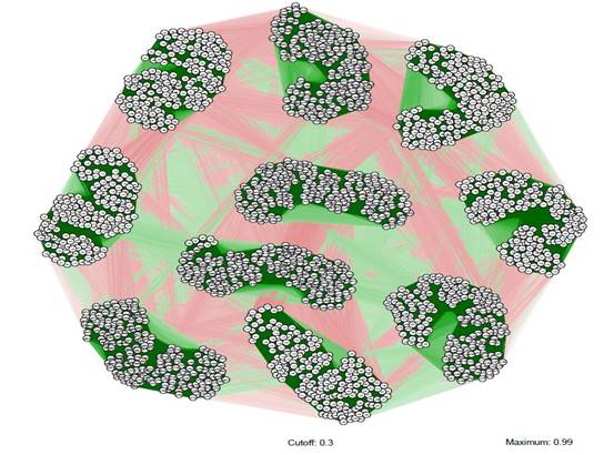
Eight (08) response variables (Yᵢ with i = 1,..,8) with predetermined mean values and heritability were considered. The heritability values ranged from 20% to 80%. Additionally, 2010 predictor variables representing molecular information in the form of SNP (Single Nucleotide Polymorphism) markers were generated. Figure 1 illustrates the correlation matrix of these 2010 variables, revealing blocks of associations representing gene linkages established by groups of 201 markers distributed across ten linkage groups or basic chromosomes of the simulated species.

Each marker was encoded with values of 2, 1, and 0, representing a discrete multicategory variable. These markers exhibited the expected Mendelian segregation in a 1:2:1 ratio. They were distributed across a genome consisting of 10 linkage groups, mirroring the genetic structure of a diploid species with 2n = 2x = 20 chromosomes. Each linkage group spanned a length of 100 centimorgans and contained 201 markers evenly spaced.

The continuous response variables followed normal distributions and were influenced by environmental effects of varying magnitude. They were determined by the action of alleles from either 40 or 44 QTLs (Quantitative Trait Loci) selected from among the 2010 previously genotyped markers. These QTLs had differential additive effects and weights denoting their importance in the total genotypic variability of the trait. These weights were established based on a uniform distribution.

Figure 1
Correlation matrix 2010x2010 of predictor variables (SNPs).

The dataset in this study was divided into two parts, namely the training and validation sets, using the K-Fold Cross-Validation method. As suggested by James et al. (2021), this division entails: a) the first part of the dataset is allocated for training purposes, where predictors are generated; b) the second part of the dataset is reserved for validation, assessing the predictive capability of the model by employing the predictor generated in the first part to make predictions for Y using the data from this second part. This approach is commonly employed when the objective is to evaluate the efficiency of prediction models or validation techniques, which is the primary focus of this study.

In the K-Fold Cross-Validation method, the sample of size n is divided into k parts or K-Folds, with the training sample obtained from the remaining k-1 parts. Consequently, after k iterations, all the data is used for both training and validation purposes (Burman, 1989). Each of the nine (9) techniques presented in this article was implemented with Cross-Validation, employing a value of k equal to 5 (k = 5).

The predictive efficiency of the models was quantified using selective accuracy, or the coefficient of determination (R²), calculated as the simple mean of the estimates for each fold (k) in each fitted model. Cruz (2005) stated that selective accuracy can be defined in various ways. In Quantitative Genetics, this measure is described as the square of the correlation between the estimated values and the true values. It represents the degree to which the obtained estimate is related to the true value of the parameter, as shown in the equation:

${\mathrm{R}}^2={\left(\mathrm{c}\mathrm{o}\mathrm{r}\left(\widehat{\mathrm{y}},\mathrm{y}\right)\right)}^2$

where: ŷ represents the predicted values generated by the model in both the training and validation sets and y represents the observed values.

Results and discussion

The results of the prediction models were obtained, considering various factors. Each model used eight response variables, subject to different noise levels (0.20, 0.40, 0.60, and 0.80), and the influence of two groups of markers (40 and 44). Additionally, a 5-fold Cross-Validation approach (k = 5) was employed, dividing the data into five sets (80% for training and 20% for validation). The selection metric used was the mean validation R² value across these five datasets.

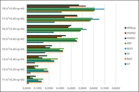
The results of the fitted models are presented in Table 1. The top three prediction models were RBF, BAG, and BOO. When examining Figure 2, it becomes clear that predictive accuracy increases as noise decreases, which corresponds to higher heritability values. In simpler terms, response variables with higher noise levels tend to yield lower R² values for all nine models considered.

Further investigation of noise levels in response variables (Figure 2) reveals that, for high noise levels in the data (0 to 0.50 range), RBF (Y₁, Y₃, and Y₄) and BAG (Y₂) exhibited the highest predictive efficiency⁷. Conversely, for low noise levels in the data (0.50 to 0.80 range), RBF (Y₅) and BOO (Y₆, Y₇, and Y₈) demonstrated the highest predictive efficiency.

Table 1
Prediction Models (mean validation R² values and k = 5).

Label / Model	DT	BAG	RF	BOO	MLP	RBF	MARS1	MARS2	RRBlup
Y1 (h²=0.20, ng=40)	0.0201	0.1376	0.1310	0.1023	0.0545	0.1471	0.0564	0.0300	0.0811
Y2 (h²=0.20, ng=44)	0.0341	0.1948	0.1908	0.1519	0.0666	0.1851	0.0774	0.0650	0.1041
Y3 (h²=0.40, ng=40)	0.0730	0.2463	0.2463	0.2174	0.1066	0.2781	0.1408	0.1072	0.1833
Y4 (h²=0.40, ng=44)	0.1646	0.3260	0.3256	0.2960	0.1356	0.3328	0.2101	0.1665	0.2268
Y5 (h²=0.60, ng=40)	0.1504	0.4545	0.4484	0.4355	0.2317	0.4568	0.2726	0.3148	0.3502
Y6 (h²=0.60, ng=44)	0.2424	0.4776	0.4860	0.5370	0.2971	0.5024	0.3721	0.3855	0.3981
Y7 (h²=0.80, ng=40)	0.2496	0.5647	0.5751	0.6523	0.3362	0.5893	0.3394	0.4560	0.4513
Y8 (h²=0.80, ng=44)	0.3129	0.6035	0.6104	0.6966	0.3450	0.6096	0.3836	0.5306	0.4686

• Note: DT (Decision Tree), BAG (Bootstrap Aggregating), RF (Randon Forest), BOO (Boosting), MLP (Multi-Layer Perceptron), RBF (Radial Basis Function Network), MARS1 and MARS2 (Multivariate Adaptative Spline linear and interacting), and RRBlup (Ridge Regression Best Linear Unbiased Predictor).

Additionally, a few general considerations about the model estimates (9) should be noted. The inclusion of 'major gene effect markers' (40 versus 44 markers) enhanced predictive efficiency. The choice of the Cross-Validation parameter (k = 5) with a relatively small sample size (1,000) and a fixed k model warrants further reflection in future studies. Numerous studies advocate for a value of k = 10 as it strikes a balance between computationally intensive fitting procedures and the bias-variance trade-off (Kim, 2009; James et al., 2021). However, as k increases, the fraction of data allocated for validation decreases, potentially compromising representativeness and predictive efficiency.

Figure 2
Prediction accuracy (R ² ) achieved by different techniques for variables with differences in gene control and environmental influence. DT (Decision Tree), BAG (Bootstrap Aggregating), RF (Randon Forest), BOO (Boosting), MLP (Multi-Layer Perceptron), RBF (Radial Basis Function Network), MARS1 and MARS2 (Multivariate Adaptative Spline linear and interacting), and RRBlup (Ridge Regression Best Linear Unbiased Predictor).

It is worth noting that techniques grouped under the same paradigm exhibited significantly different performances (e.g., MLP versus RBF or DT versus refinements). A more in-depth understanding of the dataset's statistical issues (nonlinearity, multicollinearity, and dimensionality) on each model's performance can provide insights into these variations.

In summary, when faced with the task of selecting an approach for analyzing SNP datasets, experienced biometricians may opt for tree-based models. These models are particularly well-suited for data that mirrors gene action in genetic mechanisms involving biosynthetic pathways characterized by step-by-step formation of trait-determining products. Furthermore, the binary partitions and splits inherent in tree-building procedures can effectively represent relationships between alleles within the same gene (dominance) or between different genes (epistasis). This underscores the importance of domain-specific knowledge in model selection.

However, it is crucial to emphasize that choosing an appropriate model for predicting genetic data should not rely solely on domain-specific knowledge. While valuable, other factors such as problem complexity, dataset size and quality, algorithm characteristics, and data-handling capabilities must also be considered. Therefore, while tree-based models hold promise, it is advisable to explore various approaches and modeling techniques, including linear models, neural networks, or machine learning-based methods, to determine which model best fits the dataset and analysis objectives. Model selection should be based on experimentation and rigorous result evaluation.

Conclusion

In this study, the selective accuracy of nine prediction models was evaluated in the context of data presenting statistical challenges (nonlinearity, multicollinearity, and data dimensionality), varying noise levels (heritability values of 0.20, 0.40, 0.60, and 0.80), and specificities associated with Genome-Wide Selection (GWS). Among these models, two stood out as the best fits for the simulated dataset, exhibiting the highest selective accuracy for the response variables: RBF and BOO. RBF, associated with the computational intelligence paradigm or neural network, demonstrated the highest selective accuracy in the presence of high data noise (with an honorable mention of the BAG model in Y₂). On the other hand, BOO, aligned with the tree paradigm, excelled in low-noise data settings (or high heritability scenarios). A significant generalization was drawn as follows: as data noise decreases, predictive efficiency increases for all considered models, indicating a positive correlation between heritability and selective accuracy. Our study also identified a question worthy of future research: the impact of sample size versus the value of k in the K-Fold Cross-Validation method on selective accuracy. Given the relatively small sample size in this study (1,000 individuals) and the use of k = 5, these factors may have introduced issues related to representativeness (statistical and genetic) in dataset partitioning, which should be further explored in future works concerning SNP analysis.

Acknowledgements

This study received partial funding from the Coordination for the Improvement of Higher Education Personnel (CAPES) - Finance Code 001. We extend our gratitude to the Federal University of Viçosa (UFV) and the Federal Institute of Southeast Minas Gerais (IFSEMG).

References

• Azodi, C. B., Bolger, E., McCarren, A., Roantree, M., De Los Campos, G., & Shiu, S.-H. (2019). Benchmarking oarametric and machine learning models for genomic prediction of complex traits. G3 Genes|Genomes|Genetics, 9(11), 3691-3702. DOI: https://doi.org/10.1534/g3.119.400498
  » https://doi.org/https://doi.org/10.1534/g3.119.400498
• Breiman, L. (1996). Bagging predictors. Machine Learning, 24(2), 123-140. DOI: https://doi.org/10.1007/BF00058655
  » https://doi.org/https://doi.org/10.1007/BF00058655
• Burman, P. (1989). A comparative study of ordinary cross-validation, v-fold cross-validation, and the repeated learning-testing methods. Biometrika, 76(3), 503-514. DOI: https://doi.org/10.2307/2336116
  » https://doi.org/https://doi.org/10.2307/2336116
• Costa, W. G., Celeri, M. O., Barbosa, I. P., Silva, G. N., Azevedo, C. F., Borém, A., ... Cruz, C. D. (2022). Genomic prediction through machine learning and neural networks for traits with epistasis. Computational and Structural Biotechnology Journal, 20, 5490-5499. DOI: https://doi.org/10.1016/j.csbj.2022.09.029
  » https://doi.org/https://doi.org/10.1016/j.csbj.2022.09.029
• Cruz, C. D. (2005). Princípios de genética quantitativa Viçosa, MG: UFV.
• Cruz, C. D., Salgado, C. C., & Bhering, L. L. (2013). Genômica aplicada Visconde do Rio Branco, MG: Suprema.
• Cruz, C. D. (2016). Genes Software - extended and integrated with the R, Matlab and Selegen. Acta Scientiarum. Agronomy, 38(4), 547-552. DOI: https://doi.org/10.4025/actasciagron.v38i4.32629
  » https://doi.org/https://doi.org/10.4025/actasciagron.v38i4.32629
• Cruz, C. D., & Nascimento, M. (2018). Inteligência computacional aplicada ao melhoramento genético Viçosa, MG: UFV.
• Endelman, J. B. (2011). Ridge regression and other kernels for genomic selection with R Package rrBLUP. The Plant Genome, 4(3), 250-255. DOI: https://doi.org/10.3835/plantgenome2011.08.0024
  » https://doi.org/https://doi.org/10.3835/plantgenome2011.08.0024
• Ghafouri-Kesbi, F., Rahimi-Mianji, G., Honarvar, M., & Nejati-Javaremi, A. (2017). Predictive ability of random forests, boosting, support vector machines and genomic best linear unbiased prediction in different scenarios of genomic evaluation. Animal Production Science, 57(2), 229-236. DOI: https://doi.org/10.1071/AN15538
  » https://doi.org/https://doi.org/10.1071/AN15538
• Hastie, T., Tibshirani, R., & Friedman, J. H. (2009). The elements of statistical learning: Data mining, inference, and prediction (2nd ed). Berlin, GE: Springer.
• Haykin, S. S. (2009). Neural networks and learning machines (3rd ed). New Jersey, NY: Prentice Hall.
• Izbicki, R., & Santos, T. M. (2020). Aprendizado de máquina: Uma abordagem estatística São Carlos, SP: Rafael Izbicki. Retrieved on Feb. 10, 2023 from 10, 2023 from http://www.rizbicki.ufscar.br/AME.pdf
  » http://www.rizbicki.ufscar.br/AME.pdf
• James, G., Witten, D., Hastie, T., & Tibshirani, R. (2021). An introduction to statistical learning: With applications in R (2nd ed.). Berlin, GE: Springer. DOI: https://doi.org/10.1007/978-1-0716-1418-1
  » https://doi.org/https://doi.org/10.1007/978-1-0716-1418-1
• Kim, J.-H. (2009). Estimating classification error rate: Repeated cross-validation, repeated hold-out and bootstrap. Computational Statistics & Data Analysis, 53(11), 3735-3745. DOI: https://doi.org/10.1016/j.csda.2009.04.009
  » https://doi.org/https://doi.org/10.1016/j.csda.2009.04.009
• LeCun, Y., Bengio, Y., & Hinton, G. (2015). Deep learning. Nature, 521(7553), 436-444. DOI: https://doi.org/10.1038/nature14539
  » https://doi.org/https://doi.org/10.1038/nature14539
• Li, B., Zhang, N., Wang, Y.-G., George, A. W., Reverter, A., & Li, Y. (2018). Genomic prediction of breeding values using a subset of snps identified by three machine learning methods. Frontiers in Genetics, 9(237), 1-20. DOI: https://doi.org/10.3389/fgene.2018.00237
  » https://doi.org/https://doi.org/10.3389/fgene.2018.00237
• Meuwissen, T. H., Hayes, B. J., & Goddard, M. E. (2001). Prediction of total genetic value using genome-wide dense marker maps. Genetics, 157(4), 1819-1829. DOI: https://doi.org/10.1093/genetics/157.4.1819
  » https://doi.org/https://doi.org/10.1093/genetics/157.4.1819
• Montesinos López, O. A., Montesinos López, A., & Crossa, J. (2022). Multivariate statistical machine learning methods for genomic prediction Berlin, GE: Springer International Publishing. DOI: https://doi.org/10.1007/978-3-030-89010-0
  » https://doi.org/https://doi.org/10.1007/978-3-030-89010-0
• Park, J., & Sandberg, I. W. (1991). Universal approximation using radial-basis-function networks. Neural Computation, 3(2), 246-257. DOI: https://doi.org/10.1162/neco.1991.3.2.246
  » https://doi.org/https://doi.org/10.1162/neco.1991.3.2.246
• Prasad, A. M., Iverson, L. R., & Liaw, A. (2006). newer classification and regression tree techniques: bagging and random forests for ecological prediction. Ecosystems, 9(2), 181-199. DOI: https://doi.org/10.1007/s10021-005-0054-1
  » https://doi.org/https://doi.org/10.1007/s10021-005-0054-1

• 1
  This relationship can be presented in terms of variance (VF = VG + EV) and heritability can be defined from this equation as: h² = VG/VF (how much of the total variance is genetic variance).
• 2
  This item provides a brief overview of the nine models used without delving into the specifics of mathematics, parameter setting, or algorithm tuning. Additionally, it presents some fundamental issues to be considered and suggestions for references for the deepening of each model.
• 3
  The effect of the λ penalty function is more easily noticeable in the matrix notation of the RR-Blup model.
• 4
  Nonlinearity in Biometrics is associated with the term epistasis, which is a genetic term to designate the interaction between alleles of different loci that, besides the additive-dominant effects, determines the genotypic expression of a character.
• 5
  In this study, the activation function used was the hyperbolic tangent, defined by the following equation: <mml:math><mml:mi mathvariant="normal">t</mml:mi><mml:mi mathvariant="normal">a</mml:mi><mml:mi mathvariant="normal">n</mml:mi><mml:mi mathvariant="normal">h</mml:mi><mml:mi mathvariant="normal"> </mml:mi><mml:mi mathvariant="normal">x</mml:mi><mml:mi mathvariant="normal"> </mml:mi><mml:mo>=</mml:mo><mml:mi mathvariant="normal"> </mml:mi><mml:mfrac><mml:mrow><mml:mn>1</mml:mn><mml:mo>-</mml:mo><mml:msup><mml:mrow><mml:mi mathvariant="normal">e</mml:mi></mml:mrow><mml:mrow><mml:mo>-</mml:mo><mml:mn>2</mml:mn><mml:mi mathvariant="normal">x</mml:mi></mml:mrow></mml:msup></mml:mrow><mml:mrow><mml:mn>1</mml:mn><mml:mo>+</mml:mo><mml:msup><mml:mrow><mml:mi mathvariant="normal">e</mml:mi></mml:mrow><mml:mrow><mml:mo>-</mml:mo><mml:mn>2</mml:mn><mml:mi mathvariant="normal">x</mml:mi></mml:mrow></mml:msup></mml:mrow></mml:mfrac></mml:math>.
• 6
  Radial functions are a special class of functions whose value decreases or increases concerning the distance from a central point.
• 7
  In the context of this article, predictive efficiency is indeed synonymous with selective accuracy. It is quantified by calculating the mean R² value across five validation sets.

Publication Dates

• Publication in this collection
  25 Oct 2024
• Date of issue
  2024

History

• Received
  19 June 2023
• Accepted
  27 Oct 2023