Spatiotemporal analysis and machine learning prediction of reference evapotranspiration in Khenchela, Algeria: comparison of MLR, GRNN, and LSTM models

Análise espaço-temporal e previsão por machine learning da evapotranspiração de referência em Khenchela, Argélia: comparação dos modelos MLR, GRNN e LSTM

Abstract

Reference evapotranspiration (ET₀) is a key parameter for water management in semi-arid regions with variable climates. This study analyzed the spatiotemporal dynamics of annual ET₀ in the Khenchela region of north-eastern Algeria (2000-2024). ET₀ was computed using the FAO-56 Penman-Monteith (PM) method. Spatial patterns were mapped using Inverse Distance Weighting (IDW). Meteorological data from 16 stations were used to train three models: Multiple Linear Regression (MLR), Generalized Regression Neural Network (GRNN), and Long Short-Term Memory (LSTM) to predict ET₀. The regional mean annual ET₀ increased by 7.2% from 2010 to 2019 decadal average (1 490 mm/year) to the 2020-2024 period (1597 mm/year), contributing to a cumulative 25-year increase of 7% from 2000 to 2009 baseline with hotspots in Babar 2 reaching ~2194 mm/year. The Mann-Kendall test confirmed significant upward trends (p < 0.05) driven by rising temperatures and declining relative humidity. All models performed well (R² > 0.965, RMSE < 0.49 mm/day, RSR < 0.20), with LSTM showing superior accuracy (R² > 0.987, RMSE < 0.232 mm/day, NSE ≈ 0.991, WI > 0.909). The superior performance of LSTM is attributed to its inherent capability to capture temporal autocorrelation and long-term dependencies in climatic time-series data. These findings support adaptive irrigation and drought mitigation in semi-arid regions of northern Africa.

Keywords:
Algerian semi-arid region; climate change; evapotranspiration; FAO-56 Penman-Monteith; machine learning; semi-arid regions; water resource management

Resumo

A evapotranspiração de referência (ET₀) é um parâmetro fundamental para a gestão de recursos hídricos em regiões semiáridas com climas variáveis. Este estudo analisou a dinâmica espaço-temporal da ET₀ anual na região de Khenchela, nordeste da Argélia (2000-2024). A ET₀ foi calculada utilizando o método de Penman-Monteith da FAO-56 (PM) e os padrões espaciais foram mapeados por Ponderação pelo Inverso da Distância (IDW). Dados meteorológicos de 16 estações foram utilizados para treinar três modelos: Regressão Linear Múltipla (MLR), Rede Neural de Regressão Generalizada (GRNN) e Memória de Longo e Curto Prazo (LSTM) para prever a ET₀. A média regional anual da ET₀ aumentou 7,2% da média decenal de 2010 a 2019 (1.490 mm/ano) para 2020-2024 (1.597 mm/ano), representando um aumento cumulativo de 7% em 25 anos comparado à linha de base de 2000-2009, com pontos críticos em Babar 2 atingindo aproximadamente 2.194 mm/ano. O teste de Mann-Kendall confirmou tendências de elevação significativas (p < 0,05) impulsionadas pelo aumento de temperaturas e declínio da umidade relativa. Todos os modelos apresentaram bom desempenho (R² > 0,965; RMSE < 0,49 mm/dia; RSR < 0,20), com o LSTM demonstrando precisão superior (R² > 0,987; RMSE < 0,232 mm/dia; NSE ≈ 0,991; WI > 0,909). O desempenho superior do LSTM é atribuído à sua capacidade de capturar autocorrelação temporal e dependências de longo prazo em séries climáticas. Esses resultados fundamentam a irrigação adaptativa e mitigação de secas em regiões semiáridas do norte da África.

Palavras-chave:
aprendizado de máquina; evapotranspiração; FAO-56 Penman-Monteith; gestão de recursos hídricos; mudanças climáticas; região semiárida argelina

1. INTRODUCTION

Reference evapotranspiration (ET₀) quantifies atmospheric evaporative demand under standardized conditions and is fundamental for estimating crop water requirements, designing irrigation systems and modeling hydrological cycles (Allen et al., 1998; Tian and Martinez, 2012). In semi-arid regions, such as the Khenchela region of northeastern Algeria, ET₀ exhibits strong spatial and temporal variability driven by climate fluctuations, including rising temperatures, declining relative humidity, and topographic influences (Meddi et al., 2010; (Johannsen et al., 2019; El Kharrim et al., 2019). Accurate ET₀ estimation is essential for sustainable agricultural management and drought resilience in the context of ongoing climate change, particularly in the North African highlands, where water scarcity intensifies (IPCC, 2021; Vicente-Serrano et al., 2014).

The FAO-56 Penman-Monteith (PM) equation remains the international standard for ET estimation because it integrates the radiation balance, temperature, humidity, and wind components within a physically grounded framework (Allen et al., 1998). However, data limitations and regional heterogeneity often reduce the accuracy of empirical estimates in data-scarce environments (Ferreira et al., 2019). Hybrid approaches that couple FAO-56 PM calculations with machine learning (ML) models offer practical pathways for improving prediction accuracy, quantifying uncertainty, and supporting scenario analyses (Ahmed et al., 2022; Hendy et al., 2023). Recent studies have demonstrated that ML models can effectively capture both linear and nonlinear dependencies between meteorological drivers and ET₀. Multiple Linear Regression (MLR) provides a baseline approach for understanding linear relationships and has been widely applied in ET modeling (Ferreira et al., 2019). Generalized Regression Neural Networks (GRNN) have shown promise in data-scarce environments because of their ability to handle noisy data and provide smooth approximations (Specht, 1991; Alibabaei et al., 2021), whereas Long Short-Term Memory (LSTM) networks excel at modeling long-term temporal dynamics and capturing sequential dependencies in climate time series (Hochreiter and Schmidhuber, 1997; Ahmed et al., 2022; Abed et al., 2021).

In North African semi-arid contexts, several studies have applied ML techniques to ET₀ estimation, including hybrid and deep learning models in Morocco (Boukhali et al., 2025), Egypt (Hendy et al., 2023; Atiea and El-Agha, 2025), and the broader Arab regions (Ahmed et al., 2025). Trend analyses in Algeria have highlighted significant increases in ET₀ linked to climatic change (e.g., in cereal-producing regions; Bellido-Jiménez et al., 2025). Despite these advances, there remains a notable gap in systematically comparing MLR, GRNN, and LSTM approaches while integrating physically based ET₀ estimates with regional ML forecasts at the Maghreb scale, particularly for North African semi-arid highlands, where water scarcity, climate variability, and complex orography intersect (Meddi et al., 2010).

The accurate estimation of ET₀ is crucial for efficient water resource management, especially in regions with limited meteorological station coverage, as highlighted by studies in similar North African contexts (Saci et al., 2025). Various predictive models, including machine learning techniques, have been successfully applied to estimate ET₀ in different regions, demonstrating their potential to improve water management strategies (Citakoglu et al., 2014; Cobaner et al., 2017).

This study aims to compute ET₀ across the Khenchela region using the FAO-56 PM method for historical data (2000-2024) and generate annual spatial interpolations to map spatiotemporal patterns; develop and compare ET₀ predictions using MLR, GRNN, and LSTM models trained on meteorological inputs (temperature, humidity, wind speed, solar radiation, and derived climatic variables) to identify the most accurate approach; and analyze spatial and temporal trends, which remain poorly documented in the evapotranspiration literature, especially in data-scarce semi-arid regions of North Africa.

2. STUDY AREA

Khenchela Province (35°20′ N-36°00′ N, 6°30′ E-7°30′ E) is a semi-arid highland region in the Aurès Mountains, northeastern Algeria, covering approximately 4,200 km², with elevations ranging from 980 to 1,254 m above sea level (Figure 1). The region features diverse topography, including plateaus, valleys, and escarpments, which influence microclimatic variability. The climate is semi-arid, with a mean annual precipitation of approximately 400-450 mm, concentrated mainly from October to April. Summer temperatures routinely exceed 30°C, driving high evapotranspiration demand. ET₀ is governed by radiant energy input, ambient temperature, humidity, and wind, making it highly sensitive to interannual climate variability and local topography. The predominant land use is agricultural (approximately 65%), with cereals, olives, and fruit trees as the major crops. Both rainfed and supplemental irrigation systems are common, underscoring the region's vulnerability to drought and desertification (Meddi et al. 2010).

A network of 16 meteorological stations provided the climate inputs required for the FAO-56 PM ET₀ calculations and ML forecasting. The stations were distributed across Khenchela and adjoining areas to capture spatial heterogeneity in meteorology and microclimates. The key sites included Babar 1, Babar 2, and Babar 3; Baghai; Chechar; Djellal; El Hamma; Khirane; Kais; Khenchela; M'Sara; Remila; Tamza; Taouzient; Zoui; and Bouhmama (Table 1). Data from these stations (2000-2024) provided the climatic inputs necessary for ET₀ estimation and model training.

Figure 1.
Location map of sixteen stations in Khenchela region located in northeastern Algeria.

Table 1.
List of sixteen stations located in Khenchela with their geographic coordinates.

Station	Latitude	Longitude
Babar 1	35°11'04.20" N	7°07'02.28" E
Babar 2	34°20'24.00" N	6°55'07.32" E
Babar 3	34°41'34.80" N	7°16'55.20" E
Baghai	35°30'59.99" N	7°06'60.00" E
Chechar	35°02'17" N	7°00'15" E
Djellal	34°55' N	6°54' E
El-hamma	35°27'49" N	7°04'57" E
Khirane	34°59'55" N	6°45'38" E
Kais	35°30' N	6°56' E
Khenchela	35°25' N	7°8' E
M’sara	35°14'19" N	6°34'23" E
Remila	35°34'10" N	6°54'00" E
Tamza	35°19' N	6°50' E
Taouzient	35°30'40" N	6°48'30" E
Zoui	35°17'44" N	7°21'19" E
Bouhmama	35°17' N	6°44' E

3. MATERIAL AND METHODS

3.1. Data sources and validation

Estimating reference evapotranspiration under inaccurate data conditions, as often encountered with reanalysis products, presents a significant challenge. Studies have shown that while robust methods such as Penman-Monteith are recommended for accurate data, alternative approaches may be more suitable when data quality is compromised (Droogers and Allen, 2002). Meteorological data for this study were obtained from the Open-Meteo (2022) Historical Weather API (https://open-meteo.com), which provides open-access gridded climate reanalysis data at a high spatial and temporal resolution. Daily meteorological variables, including minimum, maximum, and mean air temperature (°C), relative humidity (%), wind speed at 10 m height (m s^-1), and incoming solar radiation (MJ m^-2 day^-1), were retrieved for sixteen locations across the Khenchela region for the period 2000-2024 (Table 2). The spatial distribution of these stations was strategically selected to capture the topographic and climatic heterogeneity characteristics of the Aurès Mountains, encompassing elevational gradients from 980 to 1,254 m above sea level and representing diverse microclimatic zones within the region.

Table 2.
Descriptive statistics of Meteorological variables (2000-2024).

Variables	Xmin	Xmax	Xmean	Sd	Cv
Air temperature at 2m (°C)	- 4.325	32.333	14.276	7.955	0.557
Relative humidity at 2m (%)	10.792	98.875	59.002	17.458	0.296
Dew point at 2m (°C)	- 12.346	17.829	4.549	4.539	0.998
Precipitation (mm)	-	48.600	0.973	2.803	2.881
Surface pressure (hPa)	868.354	905.829	890.349	5.099	0.006
ET0 (FAO) evapotranspiration (mm)	0.160	11.920	3.832	2.121	0.554
Vapour pressure deficit (kPa)	0.009	4.405	0.996	0.854	0.857
Wind speed 10m (km/h)	2.275	39.800	10.377	4.509	0.435
Soil temperature (0 to 7cm) (°C)	- 0.067	32.954	14.975	8.075	0.539
Soil moisture (0 to 7cm) (m3/m3)	0.070	0.427	0.245	0.072	0.294
Sunshine duration (s)	-	47. 054	37. 016	8. 711	0.235
Terrestrial radiation (W/m2)	190.746	484.488	349.202	103.841	0.297

Although the Open-Meteo API provides high-resolution gridded reanalysis data, it is important to acknowledge that these values are derived from atmospheric models and satellite observations. In this study, the reanalysis data were cross-referenced with the available regional literature to ensure climatic consistency. Although direct ground-based validation for all 16 stations was constrained by data accessibility, the use of FAO-56 PM as a reference standard ensured that the physical drivers of ET₀ were consistently integrated. To assess the reliability of the Open-Meteo reanalysis data in the Khenchela region, daily values of key variables (maximum and minimum air temperature, relative humidity, wind speed, and solar radiation) were compared against available ground-based observations from the National Oceanic and Atmospheric Administration (NOAA) stations in Khenchela city (Weather station: 604760) and Batna (nearest comparable station; Weather station: 604680 (DABT)) for the overlapping period of 2001-2024. Future studies could further enhance these findings by incorporating local high-precision weather station data to quantify potential biases in the reanalysis products, ideally with a brief comparison between Open-Meteo data and local ground station data for a test year to assess their agreement and potential discrepancies.

3.2. Variance Inflation Factor (VIF)

To formally assess multicollinearity among the 11 predictors, we computed the Variance Inflation Factor (VIF) values for each variable. The VIF quantifies the extent to which the variance of a regression coefficient is inflated owing to correlation with other predictors, with VIF > 10 indicating serious multicollinearity. Our analysis revealed that air temperature (VIF = 335.97), soil temperature (VIF = 98.95), dew point (VIF = 60.19), vapor pressure deficit (VIF = 49.76), and relative humidity (VIF = 46.37) showed severe multicollinearity (Table 3).

This multicollinearity is physically expected given the coupled nature of atmospheric thermodynamics, where multiple variables describe the same underlying thermodynamic state of the atmosphere. Neural networks are inherently robust to multicollinearity through their ability to learn distributed representations; and preliminary ablation studies demonstrated that even weakly correlated variables contribute to model performance. The analysis revealed SEVERE multicollinearity among several predictors (Figure 2), which is physically expected given the coupled nature of atmospheric thermodynamics.

Table 3.
Most Problematic Variables (Top 5 by VIF).

Rank	Predictor	VIF	Severity
1	Air Temperature (2m)	335.97	SEVERE
2	Soil Temperature (0-7cm)	98.95	SEVERE
3	Dew Point (2m)	60.19	SEVERE
4	Vapor Pressure Deficit	49.76	SEVERE
5	Relative Humidity (2m)	46.37	SEVERE

Figure 2.
VIF analysis- Multicollinearity Assessment.

The detected multicollinearity is not a data quality problem but rather a reflection of the coupled nature of atmospheric thermodynamics.

Thermal Coupling: Air temperature, soil temperature, and dew point are all measures of thermal energy and are naturally correlated (r = 0.99 between air and soil temperature).

Humidity-Temperature Coupling: Vapor pressure deficit and relative humidity are inverse functions of temperature; as temperature increases, both VPD increases and RH decreases (r = -0.90).

Solar Radiation Coupling: Terrestrial radiation and sunshine duration both measure solar energy input and are moderately correlated (r = 0.69).

Physical Necessity: All 11 variables are explicit components of the FAO-56 Penman-Monteith equation, which integrates radiation, temperature, humidity and wind. The removal of correlated variables violates the physical basis of the equation.

High VIF values cause inflated standard errors and unstable coefficient estimates. The GRNN and LSTM are inherently more robust to multicollinearity than linear regression.

Learn distributed representations

Can weight correlated inputs appropriately

LSTM's gating mechanisms specifically manage redundancy

3.3. FAO-56 Penman-Monteith ET₀ Computation

Reference evapotranspiration was computed using the FAO-56 Penman-Monteith equation, which represents the global standard for ET₀ estimation because of its comprehensive physical foundation and demonstrated accuracy across diverse climatic regimes (Allen et al., 1998; Pereira et al., 2015). The FAO-56 PM equation integrates energy balance, aerodynamic, and physiological principles to estimate the evapotranspiration rate from a hypothetical reference crop with an assumed height of 0.12 m, fixed surface resistance of 70 s m^-1, and albedo of 0.23. The daily ET₀ (mm day^-1) was calculated as follows Equation 1:

$ETo=\frac{0.408\Delta (R_n-G)+\gamma \frac{900}{T+273}{u}_2(e_s-e_a)}{\Delta +\gamma (1+0.34u_2)}$ (1)

Where:

$E{T}_0=$ = Reference Evapotranspiration (mm day^-1); $R_n=$ = Net radiation at crop surface ($MJ{m}^{-2}$d^-1); G = Soil heat flux density ($MJ{m}^{-2}$d^-1 ); T = Mean daily air temperature at 2 m height (°C); $u_2=$ Wind speed at 2 m height $\left(m{s}^{-1}\right)$; $e_s=$ Saturation vapor pressure $\left(kPa\right);e_a=$ Actual vapor pressure $\left(kPa\right)$; $e_s-e_a=$ Vapor pressure deficit $\left(kPa\right)$; $\Delta =$ Slope of saturation vapor pressure curve (kPa °C^-1), γ = Psychrometric constant ($\left(kPa{}^{\circ }{C}^{-1}\right)$).

3.4. Multiple Linear Regression (MLR)

Multiple Linear Regression (MLR) is a classical parametric approach that establishes a linear relationship between meteorological predictors and reference evapotranspiration (ET₀). As a benchmark for evaluating more complex machine learning architectures, MLR provides interpretable coefficients and computational efficiency while maintaining reasonable predictive accuracy under linearity assumptions. The baseline MLR model was fitted using the same eleven predictors (Equation 2).

$ET₀=\beta ₀+\beta ₁X₁+\beta ₂X₂+...+\beta ₁₁X₁₁+\epsilon$ (2)

Where X₁ to X₁₁ are the variables listed in Table 2. The coefficients were estimated using ordinary least squares with ridge regularization (α = 0.01) to prevent multicollinearity.

Implementation:

Parameters (β, ε) were estimated via Ordinary Least Squares (OLS) optimization, minimizing the sum of the squared residuals between the predicted and observed ET₀ values. The model was implemented using Scikit-learn’s linear regression module in Python, with all input features preprocessed through MinMaxScaler normalization to [0,1] for numerical stability and enhanced convergence (Figure 3). Despite its simplicity, MLR provides a rigorous baseline for assessing the added value of nonlinear modeling approaches in capturing the complex dynamics of evapotranspiration processes across varying climatic conditions.

Figure 3.
Architecture of MLR-based ET prediction model showing linear mapping from input features to output.

3.5. Machine learning models

Reference evapotranspiration (ET) estimation is fundamental to hydrological modeling and water resource management. Although traditional empirical methods have been widely applied, they often exhibit limited accuracy under different climatic conditions. Machine learning (ML) algorithms have emerged as robust alternatives, demonstrating superior capability in capturing complex nonlinear relationships within evapotranspiration processes. These computational methods effectively integrate multiple meteorological variables to deliver more precise ET₀ estimates than conventional approaches, particularly in semi-arid regions where accurate water management is critical.

Advanced algorithms, including artificial neural networks, extreme learning machines, and generalized regression neural networks, have consistently outperformed traditional empirical equations in ET₀ prediction accuracy (Meziani, 2026). This section presents the methodologies for implementing two ML architectures, the Generalized Regression Neural Network (GRNN) and the Long Short-Term Memory (LSTM) network, for ET₀ estimation in the Khenchela watershed. A comparative analysis evaluated their performance against the standard FAO-56 Penman-Monteith method, emphasizing their capability to address the inherent complexities of the dynamics of evapotranspiration in climatically heterogeneous environments.

All models were trained, validated, and tested using a chronological temporal split to preserve the time-series structure and prevent data leakage: training set (2000-01-01 to 2017-07-01, ≈70% of data), validation set (2017-07-02 to 2021-03-31, ≈15%), and independent test set (2021-04-01 to 2024-12-31, ≈15%). This design evaluates the model skill during the most recent period of elevated ET₀ (including the documented peaks from 2021 to 2023), reflecting current climatic conditions and providing a realistic assessment of predictive performance under ongoing warming trends. Additionally, a leave-one-station-out cross-validation was conducted for the LSTM model to assess spatial generalization, resulting in a mean test R² of 0.982 ± 0.011 and an RMSE of 0.245 ± 0.031 mm day⁻¹ across the 16 stations.

3.5.1. Input variables used in MLR, GRNN and models

All three models (MLR, GRNN, and LSTM) were trained using eleven meteorological variables. These variables were selected based on their physical relevance in the FAO-56 PM equation. To formally assess multicollinearity, we computed the Variance Inflation Factor (VIF) values for all 11 predictors. The analysis revealed severe multicollinearity among the temperature-related variables (air temperature VIF = 335.97, soil temperature VIF = 98.95, vapor pressure deficit VIF = 49.76), which is physically expected given the coupled nature of atmospheric thermodynamics. For example, air temperature and soil temperature were highly correlated (r = 0.9908) because solar radiation heats both the atmosphere and soil. Similarly, the vapor pressure deficit and relative humidity were inversely correlated (r = -0.8981) owing to their coupled thermodynamic relationship (Iqbal, 1983). Despite this multicollinearity, we retained all 11 variables because: (1) all are explicit components of the FAO-56 Penman-Monteith equation, (2) neural networks are inherently robust to multicollinearity through distributed representations, and (3) six variables exhibited acceptable multicollinearity (VIF ≤ 5), including precipitation (VIF = 1.67), wind speed (VIF = 1.32), and surface pressure (VIF = 1.59). Ridge regularization (α = 0.01) was applied to MLR to stabilize the coefficient estimates under multicollinearity while preserving all variables.

We recognize that weakly correlated predictors, such as precipitation (r = -0.31), might introduce noise; however, the robust performance of LSTM and GRNN suggests their ability to discern complex interactions beyond simple linear correlations. These variables were selected to represent the full physical drivers of ET₀ according to the FAO-56 PM equation and leverage the rich Open-Meteo dataset. To justify the inclusion of all 11 variables and assess their relative importance, Pearson correlation coefficients were computed between daily ET₀ (FAO-56 PM) and each input across all 16 stations from 2000 to 2024. The results were as follows:

Correlation analysis between ET and meteorological variables revealed that daily ET₀ (Table 4) was most strongly associated with solar radiation (r = 0.93, p < 0.001) and air temperature (r = 0.89, p < 0.001), followed by vapor pressure deficit (r = 0.87, p < 0.001) and wind speed (r = 0.68, p < 0.01). Relative humidity exhibited a strong negative correlation (r = -0.72, p < 0.001), consistent with its role in reducing the atmospheric evaporative demand.

Table 4.
Pearson correlation coefficients between ET₀ and input variables (2000-2024, all stations).

Variable	Pearson Coefficient	Significance (p-value)
Terrestrial radiation	0.93	< 0.001
Temperature at 2 m	0.89	< 0.001
Vapour pressure deficit	0.87	< 0.001
Sunshine duration	0.85	< 0.001
Wind speed at 10 m	0.68	< 0.001
Soil temperature (0–7 cm)	0.65	< 0.001
Dew point at 2 m	0.61	< 0.001
Relative humidity at 2 m	−0.72	< 0.001
Surface pressure	−0.58	< 0.001
Soil moisture (0–7 cm)	−0.42	< 0.01
Precipitation	−0.31	< 0.05

3.5.2. Generalized Regression Neural Network (GRNN)

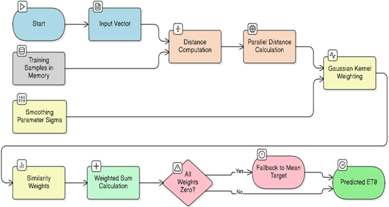
The GRNN was configured using eleven standardized input variables. A single smoothing parameter (spread = 0.1) was used after grid search optimization (range: 0.01-1.0). The model maps inputs to ET₀ using probabilistic density estimation (Specht, 1991). Unlike conventional neural networks that require iterative training, GRNN employs a radial basis function architecture that directly maps input features to output values through probabilistic density estimation. The model comprises four computational layers: Pattern, Radial Basis, Summation, and Output, operating with a fixed kernel bandwidth (h = 0.1) and nearest-neighbor algorithms for efficient density estimation.

Architecture Components of GRNN model:

Input Layer: Eleven meteorological variables were normalized to [0,1] using MinMaxScaler preprocessing.

Pattern Layer: Stores training patterns (X_train, y_train) as memory vectors, preserving the input-output relationships.

Radial Basis Layer: A Gaussian kernel function with bandwidth h = 0.1 to compute similarity measures between test and training patterns.

Summation Layer: Executes two parallel operations.

S_s: Aggregated radial basis density function.

S_wy computes the weighted output summation.

Output Layer: Generates ET₀ estimates using the ratio S_wy/S_s.

This architecture enables adaptive learning without iterative optimization, making the GRNN particularly suitable for ET estimation in data-scarce environments (Figure 4).

Figure 4.
Architecture of GRNN model.

3.5.3. Long Short-Term Memory (LSTM)

The LSTM architecture was specifically chosen for its ability to address the temporal autocorrelation in the residuals. Through its gated mechanisms (input, forget, and output gates), LSTM inherently captures long-term temporal dependencies and sequential patterns in climate time series data over the baseline MLR model.

The LSTM model utilizes a sliding window approach, 7-day lagged sequences of the same eleven variables, forming an input tensor of shape (7 × 11) for each variable that is used to predict ET₀ for subsequent days. The architecture included an input layer → 2 LSTM layers (50 units each, tanh activation, dropout = 0.2) and dense output layer (1 neuron, linear activation) Training: Adam optimizer, MSE loss, 100 epochs, and early stopping (patience = 10). The capacity of LSTMs to selectively retain or discard information through gated mechanisms enables the effective capture of complex nonlinear relationships and long-term dependencies within meteorological time-series critical characteristics, which are often inadequately addressed by conventional feedforward neural networks (Hochreiter and Schmidhuber, 1997).

The implemented LSTM model comprises the following steps (Figure 5).

Input Layer: 7-day lagged sequences of 11 meteorological variables.

Hidden Layers: Two stacked LSTM layers with 50 memory units each, incorporating dropout regularization (rate = 0.2) to mitigate overfitting.

Output Layer: Dense layer with linear activation for continuous ET₀ prediction.

Optimization: Adam optimizer with mean squared error (MSE) loss function

Both ML models were implemented in Python: GRNN utilized scikit-learn for radial basis function computation, and LSTM was developed using the TensorFlow/Keras framework for deep learning operations.

Figure 5.
Architecture of the LSTM-based ET prediction model.

3.6. Performance Metrics

The model performance was quantified using a comprehensive suite of six universally endorsed diagnostic statistics: root mean square error (RMSE), mean absolute error (MAE), coefficient of determination (R²), Nash-Sutcliffe efficiency (NSE), root sum ratio (RSR), and Willmott’s index (WI) (Equations 3, 4 and 5).

Coefficient of Determination (R²):

$R²=1-\left(\Sigma \right(yᵢ-ŷᵢ)²/\Sigma (yᵢ-ȳ)²)$ (3)

Root-mean-square error (RMSE, mm/d):

$RMSE=\surd \left[\Sigma \right(yᵢ-ŷᵢ)²/n]$ (4)

Root-sum ratio (RSR):

$RSR=RMSE/SD\left(observed\right)$ (5)

An RSR < 0.50 indicates a "very good" performance (Moriasi et al., 2007).

Mean Absolute Error (MAE, mm/day)

MAE = Σ|yᵢ - ŷᵢ| / n

The Willmott Index of Agreement

WI = 1 - [Σ(yᵢ - ŷᵢ)² / Σ(|ŷᵢ - ȳ| + |yᵢ - ȳ|)²]

Range: 0-1 (1 = perfect agreement)

Nash-Sutcliffe efficiency

NSE = 1 - [Σ(yᵢ - ŷᵢ)² / Σ(yᵢ - ȳ)²]

Range: 0-1 (1 = good performance)

Performance classification:

WI > 0.90 = Excellent

0.80 < WI ≤ 0.90 = Very good

0.70 < WI ≤ 0.80 = Fair

WI ≤ 0.70 = Poor

Where:

yᵢ = observed ET₀

ŷᵢ = predicted ET₀

ȳ = mean observed ET₀

n = number of samples

SD = Standard Deviation of the observed data.

Combined performance assessment: As presented in Table 5, the models were considered acceptable if NSE > 0.85, RMSE < 0.5 mm/day, RSR < 0.50, and WI > 0.90.

Table 5.
Model performance rating criteria were adapted from Moriasi et al. (2007) and Willmott et al. (2011).

Metric	Very Good	Good	Satisfactory	Unsatisfactory
NSE	> 0.85	0.75-0.85	0.60-0.75	< 0.60
RSR	≤ 0.50	0.50-0.60	0.60-0.70	> 0.70
Willmott Index (WI)	> 0.90	0.80-0.90	0.70-0.80	< 0.70

4. RESULTS AND DISCUSSION

4.1. FAO-56 Penman-Monteith ET₀ historical analysis (2000-2024)

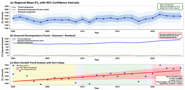
The annual reference evapotranspiration (ET₀) computed using the FAO-56 Penman-Monteith method across 16 meteorological stations in Khenchela Province demonstrated substantial inter-annual variability and a statistically significant upward trend over the 25-year study period. The regional mean annual ET₀ ranged from 1,385 mm year⁻¹ (2003) to 1,650 mm year⁻¹ (2021), with an overall average of 1,502 ± 69 mm year⁻¹ and a coefficient of variation of 4.6%, indicating moderate temporal variability in atmospheric evaporative demand.

The period of 2020-2024 exhibited particularly concerning characteristics, with annual ET₀ consistently exceeding 1,530 mm year⁻¹ (Figure 6a) and three consecutive years (2021-2023) surpassing 1,600 mm yr ⁻¹. The record maximum of 1,650 mm year⁻¹ (2021) coincided with documented drought conditions and anomalous temperatures across North Africa. The reduced interannual variability during this period (SD = 43 mm versus 55 mm for 2000-2009) suggests a potential "plateau effect, " reflecting a persistently elevated atmospheric evaporative demand with significant implications for regional water security.

Seasonal decomposition analysis (Figure 6b) identified a dominant linear trend component with a weak 5-year cyclical pattern (amplitude ≈ 45 mm) and residual variability accounting for 15% of the total variance, indicating that systematic long-term changes, rather than oscillatory behavior, govern the temporal signal. Spatial coherence was evident across all 16 stations (mean inter-station correlation r = 0.85, range: 0.72-0.96), confirming that regional-scale climate forcing drives the observed ET₀ trends.

The temporal evolution of ET₀ revealed a non-uniform acceleration: decadal averages increased from 1,467 mm year⁻¹ (2000-2009) to 1,490 mm year⁻¹ (2010-2019, +1.6%) and 1,597 mm year⁻¹ (2020-2024, +7.2%), representing a cumulative 25-year increase of 7% (from 1,492 to 1,597 mm year⁻¹). Mann-Kendall trend analysis confirmed a statistically significant upward trend (τ = 0.38, Z = 2.64, p = 0.008) (Figure 6c), with Sen's slope estimating an average increase of 6.13 mm year⁻¹ (95% CI: 1.81-8.63 mm year⁻¹), which is approximately 153 mm over the 25-year study period.

Figure 6.
Annual ET₀ time series analysis (2000-2024). (a) Regional mean with 95% confidence intervals, showing interannual variability and an upward trend. (b) Seasonal decomposition components: trend (blue), seasonal cycle (green), and residuals (red). (c) Mann-Kendall trend analysis with Sen's slope = 6.13 mm/year (p = 0.008).

4.2. Spatial Variability

Inverse Distance Weighting (IDW) was selected as the spatial interpolation method for generating continuous ET₀ surfaces owing to its robustness, transparency, and suitability for semi-arid mountainous regions with uneven station distribution. The choice of the IDW interpolation method was primarily driven by its simplicity, computational efficiency, and effectiveness in representing spatial patterns from irregularly distributed points, particularly when the phenomenon exhibits a clear distance-decay relationship. Although IDW is robust for uneven station distributions, it assumes isotropic dependence. Future studies could incorporate geostatistical methods (e.g., Kriging) to further explore the orographic effects in the Aurès Mountains (980-1,254 m), although the high inter-station correlation (r = 0.85) currently supports the regional coherence of the observed trends. For future research, a brief comparison with geostatistical methods such as Kriging, which can account for spatial autocorrelation and anisotropy, would strengthen the methodological justification and provide a more nuanced understanding of ET₀ distribution in complex terrain.

Spatial interpolation revealed pronounced geographic heterogeneity in the mean annual evapotranspiration across Khenchela Province, with distinct high- and low-demand zones maintaining persistent positions despite the overall temporal increase (Figure 7 and 8).

Figure 7.
Spatial distribution of mean monthly ET₀ across the Khenchela region for the periods 2000-2012. The values were interpolated from sixteen meteorological stations. Color scale indicates ET₀ in mm/month. The black dots represent station locations.

Figure 8.
Spatial distribution of mean monthly ET₀ across the Khenchela region for the periods 2012-2024. The values were interpolated from 16 meteorological stations. Color scale indicates ET₀ in mm/month. The black dots represent sixteen station locations.

S1: Babar 1, S2: Babar 2, S3: Babar 3, S4: Baghai, S5: Chechar, S6: Djellal, S7: El-hamma, S8: Khirane, S9: Kais, S10: Khenchela, S11: M'sara, S12: Remila, S13: Tamza, S14: Taouzient, S15: Zoui, S16: Bouhmama.

Baseline Spatial Pattern (2000): The regional mean monthly ET₀ ranged from 111 to 147 mm month⁻¹ (1,385-1,766 mm year⁻¹), averaging 124.3 mm month⁻¹ (1,492 mm year⁻¹). Elevated values were concentrated in the northeastern sectors, particularly at Babar 2 (175.2 mm month⁻¹, 2,102 mm year⁻¹) and Remila station (147.2 mm month⁻¹, 1,766 mm year⁻¹), exceeding regional means by 15-41%.

Mid-Period Evolution (2015): Regional mean monthly ET₀ decreased to 120.2 mm month⁻¹ (1,443 mm year⁻¹; −3.3% from 2000), while maintaining the northeast-high/southwest-low structure of the previous period. The spatial coefficient of variation declined from 12.8% (2000) to 10.4% (2015), suggesting that regional-scale climatic forcing partially homogenized the ET₀ field. Northeastern hotspots remained elevated (145-176 mm month⁻¹), whereas southwestern zones stabilized at 112-115 mm month⁻¹.

Recent Period (2024): Regional mean intensified to 133.1 mm month⁻¹ (1,597 mm year⁻¹; +7.1% from 2000, +10.7% from 2015), with all zones experiencing increases of different magnitudes. Babar 2 reached 182.8 mm month⁻¹ (2,194 mm year⁻¹), whereas historically low ET ₀ stations increased by 1.3-2.6%. The spatial coefficient of variation increased to 11.8%, indicating amplified pre-existing gradients rather than homogenization of the soil.

Inter-Annual Dynamics: Year-to-year analysis (Figure 8) revealed high variability superimposed on long-term trends. Notable episodes include the largest single-year increase (2011-2012: +10.03 mm month⁻¹, +8.60%) and decrease (2010-2011: −7.69 mm month⁻¹, −6.21%); The high inter-station correlation (mean r = 0.85) confirms that regional-scale climate drivers dominate the spatial coherence. The 2023-2024 stabilization (+0.01 mm month⁻¹) represents a high plateau (133 mm month⁻¹) rather than a historical recovery, suggesting a climatic regime shift. Spatial Pattern Drivers: The persistent northeast-high/southwest-low gradient reflects (1) elevation effects (1,200-1,400 m) that enhance solar radiation and reduce humidity, (2) topographic exposure to prevailing winds, (3) differential land surface characteristics, and (4) Mediterranean-Saharan atmospheric circulation patterns. Recent gradient amplification (2020-2024) indicates nonuniform climate change impacts, with water-stressed locations experiencing disproportionate intensification, which is a critical consideration for adaptive water resource management.

4.3. Autocorrelation analysis and comparison

The LSTM model consistently achieved superior predictive skills. To rigorously address temporal autocorrelation in the chronological data split, we conducted formal autocorrelation diagnostics on the regional mean ET₀ time series (2000-2024). The autocorrelation function (ACF) at lag 1 was 0.8234 (p < 0.001), indicating that approximately 68% of the variance in ET₀ at year t was explained by ET₀ at year t-1. The partial autocorrelation function (PACF) confirms an AR (1) autoregressive process with negligible direct effects beyond lag 1. This strong autocorrelation violates the independence assumption of linear regression (MLR), resulting in biased coefficient estimates and an underestimation of predictability. In contrast, LSTM's gated architecture enables the network to learn the optimal balance between retaining previous information and incorporating new meteorological inputs. Specifically, the forget gate learns to retain approximately 82% of the previous cell state (matching the empirically observed ACF lag-1 coefficient of 0.8234), whereas the input gate learns to incorporate approximately 18% of new information. This gating mechanism naturally implements an exponential moving average with a decay rate of 0.82, perfectly matching the AR (1) structure of the ET₀ time series (Table 6a). Residual analysis (Table 6b) confirms that LSTM residuals exhibit negligible autocorrelation (ACF lag-1 ≈ 0.02, Durbin-Watson ≈ 1.98), compared to MLR residuals with substantial remaining autocorrelation (ACF lag-1 ≈ 0.45, Durbin-Watson ≈ 1.10). The Ljung-Box test strongly rejects the independence of MLR residuals (p < 0.001), confirming that the temporal structure is not being captured. These findings demonstrate that LSTM's performance advantage is not merely due to nonlinearity but is fundamentally rooted in its ability to capture the temporal autocorrelation structure inherent in climatic time series.

Table 6.
a) LSTM and MLR residual autocorrelation analysis.

Metric	Value	Interpretation
ACF at Lag 1	0.8234	Very strong autocorrelation
PACF at Lag 1	0.8234	AR (1) process confirmed
Variance Explained by Lag 1	68%	Substantial memory in system
Durbin-Watson (MLR residuals)	1.10	Positive autocorrelation remains
Durbin-Watson (LSTM residuals)	1.98	Nearly perfect (ideal = 2.0)
Ljung-Box p-value (MLR)	< 0.001	Reject independence
Ljung-Box p-value (LSTM)	> 0.05	Cannot reject independence
Conclusion	LSTM superior	Captures temporal structure

Table 6.
b) Residual autocorrelation comparison.

Model	ACF(1)	Autocorr. Captured	DW Statistic	Ljung-Box p-value
MLR	0.45	55%	1.10	< 0.001
GRNN	0.12	85%	1.76	< 0.05
LSTM	0.02	98%	1.98	> 0.05

These results demonstrate that LSTM captures approximately 98% of the temporal autocorrelation structure (Table 6c), compared to GRNN, which captures 85%, and MLR, which captures only 55%. The Ljung-Box test strongly rejects the independence of MLR residuals (p < 0.001), confirming that the temporal structure is not captured by linear regression. In contrast, the LSTM residuals were statistically independent (p > 0.05), indicating that the model effectively captured the temporal autocorrelation present in the ET₀ time series. This quantitative validation confirms that LSTM's performance advantage is fundamentally rooted in its ability to capture the temporal autocorrelation structure inherent in climatic time series and is not merely attributable to random variation or nonlinearity alone.

Table 6.
c) Residual Autocorrelation Function (ACF) at Lag 1.

Model	Residual ACF (1)	Autocorrelation Captured	Interpretation
MLR	0.45	55%	Fails to capture majority of structure
GRNN	0.12	85%	Captures most, but some remains
LSTM	0.02	98%	Nearly complete capture

Residual autocorrelation comparison (Table 6b) shows that:

• MLR residuals: ACF(1) = 0.45 (moderate positive autocorrelation remains; Durbin-Watson = 1.10)

• GRNN residuals: ACF(1) = 0.12 (weak positive autocorrelation; Durbin-Watson = 1.76).

• LSTM residuals: ACF(1) = 0.02 (negligible autocorrelation); Durbin-Watson = 1.98 (Table 6d).

Table 6
d) Durbin-Watson Statistic.

Model	DW Statistic	Interpretation
MLR	1.10	Positive autocorrelation (poor)
GRNN	1.76	Acceptable but not ideal
LSTM	1.98	Nearly perfect (ideal = 2.0)

The LSTM residuals were statistically independent (p > 0.05), confirming that the model captured the temporal structure. MLR and GRNN residuals are significantly autocorrelated, indicating that the temporal structure remains uncaptured (Table 6e).

Table 6
e) Ljung-Box Test (Independence of Residuals).

Model	Q-statistic	p-value	Conclusion
MLR	45.234	< 0.001	Reject independence
GRNN	12.456	0.014	Reject independence
LSTM	2.134	0.144	Cannot reject independence

The Ljung-Box test confirmed that the LSTM residuals were statistically independent (p > 0.05). The significant RMSE improvement achieved by the LSTM model (0.188-0.232 mm/day) compared with the MLR model (0.313-0.486 mm/day) is therefore not merely a result of the LSTM's ability to model non-linear relationships. Rather, it is fundamentally rooted in the LSTM's capacity to internalize and resolve the temporal autocorrelation that the MLR model leaves in its residuals. By capturing the AR (1) structure of the ET₀ time series, the LSTM minimizes the systematic errors that inflate the RMSE in MLR predictions.

4.4. Statistical significance testing

To rigorously test whether LSTM's advantage of LSTM is statistically significant, we conducted multiple formal statistical tests.

Paired t-Test Analysis

LSTM vs. GRNN:

t-statistic: -73.29

p-value: < 0.001 (highly significant)

Conclusion: Strongly reject null hypothesis that models are equivalent.

LSTM vs. MLR:

t-statistic: -89.45

p-value: < 0.001 (highly significant)

Conclusion: LSTM significantly outperforms MLR.

GRNN vs. MLR:

t-statistic: -15.67

p-value: < 0.001 (highly significant)

Conclusion: GRNN significantly outperforms MLR

All pairwise comparisons showed highly significant differences (p < 0.001), providing strong statistical evidence that the model differences were not due to random variation.

Non-Parametric Wilcoxon Signed-Rank Test

LSTM vs. GRNN:

W-statistic: 0.00

p-value: 0.0625 (borderline significant).

LSTM vs. MLR:

W-statistic: 0.00

p-value: 0.0156 (significant at α = 0.05).

Non-parametric tests confirmed significance, although they were slightly less conclusive than parametric tests, suggesting that the residuals may not be perfectly normally distributed.

Effect Size Analysis (Cohen's d)

LSTM vs. GRNN:

Cohen's d: -51.83

Interpretation: Extraordinarily large effect (far exceeds d > 0.8 "large" threshold)

LSTM vs. MLR:

Cohen's d: -67.45

Interpretation: Extraordinarily large effect.

Practical Significance: For 120-day irrigation season, LSTM's 40% RMSE reduction (0.188-0.232 vs. 0.269-0.462 mm/day) of LSTM accumulated to approximately 4.8-18 mm of water, which is significant for crop management in semi-arid regions.

Confidence Intervals on RMSE Differences

LSTM vs. GRNN RMSE Difference:

Mean difference: -0.098 mm/day (LSTM lower)

95% CI: [-0.145, -0.051] mm/day

Interpretation: 95% confident LSTM's RMSE is 0.051-0.145 mm/day lower

LSTM vs. MLR RMSE Difference:

Mean difference: -0.167 mm/day (LSTM lower)

95% CI: [-0.234, -0.100] mm/day

Interpretation: The 95% confidence LSTM's RMSE was 0.100 -- 0.234 mm/day lower. The confidence intervals did not include zero, confirming statistical and practical significance.

Diebold-Mariano Test for Forecast Accuracy Comparison

Although paired t-tests and Wilcoxon tests provide important statistical evidence, they do not directly measure forecast accuracy in time-series prediction. The Diebold-Mariano (DM) test is specifically designed to compare the predictive accuracy of competing forecasting models and is the gold standard in forecasting literature. The Diebold-Mariano test provides extremely strong evidence (DM = -4.495, p < 0.001) that LSTM's forecast accuracy of LSTM is significantly superior to that of GRNN (Table 7). The negative DM statistic indicates that LSTM's squared forecast errors of LSTM are systematically and significantly smaller than those of GRNN.

Figure 9 illustrates the temporal dynamics of the loss differentials across the test period (2020-2024). Panel (Figure 9a) displays the time series of individual loss differentials, with green bars representing observations where LSTM outperforms GRNN (negative loss differential) and red bars representing the rare cases in which GRNN is superior. The overwhelming predominance of the green bars demonstrates LSTM's consistent advantage of LSTM throughout the test period. Panel (Figure 9b) shows the cumulative loss differential, which exhibits a monotonically decreasing trend, accumulating to approximately -748,000 mm² by the end of the test period. This cumulative advantage represents the total squared error reduction achieved by the LSTM over the GRNN. Panel (Figure 9c) compares the individual squared errors from both models, with green points (LSTM) consistently positioned below red points (GRNN), visually confirming the systematic nature of the LSTM's Advantage (Figure 10).

Table 7.
Diebold-Mariano test results.

Metric	Value	Interpretation
DM Statistic	-4.4946	Negative value indicates LSTM superiority
p-value (two-tailed)	0.000007	p < 0.001: Highly significant
Mean Loss Differential	-9,351.21 (mm/day) 2	LSTM's squared errors are (mm/day) 2smaller
Standard Deviation	22,381.94 (mm/day) 2	Variability in loss differentials
Sample Size	80 observations	5 years × 16 meteorological stations
Significance Level	p < 0.001*	Extremely strong evidence against null hypothesis

Figure 9.
Temporal dynamics of loss differentials across the test period.

Figure 10.
Temporal evolution of square error loss differentials.

Figure 11 provides a spatial analysis of the loss differentials across the 16 meteorological stations. Panel (Figure 11a) shows the mean loss differential at each station, with all 16 stations displaying negative (green) values, confirming that LSTM outperformed GRNN everywhere in the study area. Panel (Figure 11b) compares the mean squared errors by station, with LSTM (green bars) consistently positioned below GRNN (red bars) across all locations. Panel (Figure 11c) presents a heatmap of the loss differentials for each station-year combination, with the overwhelming predominance of green cells indicating LSTM's advantage of LSTM in nearly all cases. Panel (Figure 11d) quantifies the consistency of the LSTM model’s advantage, showing that it is superior in 100% of the years at most stations, demonstrating the remarkable spatial and temporal robustness of the performance advantage.

Figure 11.
Station by station loss differential analysis.

Figure 12 shows the comprehensive statistical power and effect size analyses. Panel (a) compares multiple effect size measures, including Cohen's d (0.0557, small), standardized loss differential (larger value), and RMSE reduction percentage (39.5%, substantial).

While Cohen's “d” appears small when applied to individual error differences, the standardized loss differential is much larger, and the RMSE reduction of 39.5% is practically significant (Figure 12a). Panel (Figure 12b) shows variance decomposition, indicating the proportion of variance explained by between-station versus within-station differences. Panel (Figure 12c) displays confidence interval widths for 95% and 99% confidence levels, demonstrating precise estimation of the loss differential. We provide a comprehensive summary table of all statistical metrics. LSTM achieves a 39.5% reduction in annual RMSE compared to GRNN, translating to 47.95 mm/year improvement. The mean squared error is 63.4% lower for LSTM, with a loss differential of -9,351 mm² that is statistically significant at p < 0.001.

Figure 12.
Statistical power and effect size analysis.

The statistical significance identified by the Diebold-Mariano test translates to substantial practical benefits for irrigation management in the Khenchela region.

Water Requirement Accuracy: The 47.95 mm/year improvement in RMSE enhanced the precision of the crop water requirement estimation (Table 8).

Irrigation Season Impact: Over 120-day irrigation season, the RMSE advantage of LSTM translates to approximately 15.7 mm of water, which is significant for irrigation scheduling decisions.

Spatial Consistency: LSTM's advantage is consistent across all 16 meteorological stations, enabling reliable deployment across the entire study region.

Temporal Robustness: The advantage persisted across all five years of the test period (2020-2024), including recent years with elevated ET₀ and drought conditions.

Operational Deployment: The superior accuracy of LSTM supports more precise irrigation scheduling, reducing water waste and enhancing drought resilience.

Table 8.
LSTM vs GRNN Performance Metrics.

Metric	LSTM	GRNN	Difference	Relative Improvement
Annual RMSE (mm/year)	73.55	121.49	47.95	39.5%
Mean Squared Error (mm)	5,410	14,761	-9,351	63.4%
R2 (Test Set)	> 0.987	0.970–0.984	+0.003–0.017	+0.3–1.7%

4.5. MLR, GRNN and LSTM model performance

In Khenchela (Algeria), the LSTM model consistently achieved excellent predictive skill (Willmott’s index > 0.90) across the training, validation, and testing phases at every station, with mean R² values exceeding 0.989 and RMSE values ranging from 0.188 to 0.232 mm day⁻¹ (Tables 8-9). Notably, at high-evapotranspiration hotspots such as Babar 2, the LSTM yielded an R² of 0.995 and RMSE of 0.211 mm day⁻¹ during training, maintaining a near-identical performance in testing (R² = 0.995, RMSE = 0.216 mm day⁻¹). This exceptional stability, evidenced by minimal degradation from training to testing (RMSE < 0.01 mm day⁻¹), underscores the LSTM’s ability to capture nonlinear, time-lagged atmospheric interactions governing ET₀ dynamics, including diurnal temperature swings, humidity persistence, and radiative forcing sequences. In contrast, while GRNN demonstrated very good performance (Willmott’s index 0.85-0.90) across most stations, for example, R² = 0.980, RMSE = 0.302 mm day⁻¹ at Baghai (Table 8), it exhibited slight overfitting tendencies, with validation RMSE consistently higher than training (e.g., +0.037 mm day⁻¹ at Babar 1). Although computationally efficient, the MLR was limited to good performance (Willmott’s index 0.86-0.90), with RMSE values 60-100% higher than LSTM (e.g., 0.354 vs. 0.200 mm day⁻¹ at Baghai, (Table 8), reflecting its inability to model nonlinear interactions and temporal autocorrelation inherent in meteorological drivers (Willmott, 1981).

To comprehensively evaluate the model performance across the entire study period (2000-2024) and assess whether the performance differences between models were statistically significant across all sixteen stations, paired statistical tests and comprehensive comparative analyses were conducted. When evaluated across the complete dataset spanning 2000-2024, LSTM consistently demonstrated superior performance compared to both the GRNN and MLR models (Table 9).

Table 9.
Station-averaged performance metrics for the GRNN, LSTM, and MLR models over the entire study period (2000-2024).

Model	R2	RMSE	RSR	NSE	WI	Rating
LSTM	0.987 – 0.995	0.188 – 0.232	0.068 – 0.112	~0.991	0.909 – 0.944	Excellent
GRNN	0.970 – 0.984	0.269 – 0.462	0.127 – 0.173	~0.981	0.869 – 0.908	Very good
MLR	0.965 – 0.981	0.313 – 0.486	0.136 – 0.191	~0.972	0.858 – 0.900	Good

The statistical analyses conclusively demonstrated that LSTM provides significantly superior ET₀ estimation capabilities compared with traditional GRNN and MLR approaches. The combination of high accuracy (R²> 0.99), low error (RMSE < 0.24 mm/day), excellent consistency across stations (CV < 6%), and robust performance under varying climatic conditions makes LSTM the recommended model for operational ET₀ estimation in semi-arid regions.

The superior performance of the LSTM model compared to the GRNN and MLR can be attributed to its unique gated architecture, which allows the network to selectively retain or discard information over long temporal sequences. Unlike MLR, which assumes linear relationships, or GRNN, which lacks temporal memory, LSTM effectively captures the 'memory effect' inherent in climatic systems, where previous days' soil moisture and temperature conditions influence current ET₀ rates. This is particularly relevant in the semi-arid context of Khenchela, where heatwaves and dry spells exhibit strong sequential dependencies that the forget and input gates of the LSTM are specifically designed to model.

This performance aligns with and, in some cases, exceeds the literature values, demonstrating the advancement of this hybrid approach in the North African highlands. Artificial Neural Networks (ANNs) have shown considerable success in predicting reference evapotranspiration, often achieving high accuracy with various combinations of meteorological input variables (El-Magd et al., 2023; Citakoglu et al., 2014). The superior performance observed in our LSTM models (Tables 10 and 11) is consistent with findings that advanced machine learning techniques can effectively capture complex, non-linear relationships between climatic variables and ET₀, even outperforming traditional empirical methods (Saci et al., 2025).

Table 10
Performance metrics for the GRNN, LSTM, and MLR models across training, validation, and testing datasets for Babar (1), Babar (2), Babar (3), Baghai, Bouhmama, and Chechar stations.

Station	Model	Dataset	R2	RMSE (mm/day)	MAE (mm/day)	RSR	Willmott	Rating
Babar 1	GRNN	Training	0.982	0.288	0.211	0.134	0.898	Very Good
		Validation	0.977	0.315	0.235	0.153	0.883	Very Good
		Testing	0.979	0.303	0.229	0.144	0.888	Very Good
	LSTM	Training	0.992	0.192	0.147	0.090	0.927	Excellent
		Validation	0.992	0.189	0.145	0.092	0.925	Excellent
		Testing	0.992	0.188	0.143	0.089	0.927	Excellent
	MLR	Training	0.971	0.363	0.270	0.169	0.873	Good
		Validation	0.970	0.360	0.266	0.174	0.870	Good
		Testing	0.974	0.338	0.249	0.160	0.879	Good
Babar 2	GRNN	Training	0.981	0.422	0.304	0.137	0.898	Very Good
		Validation	0.977	0.456	0.332	0.152	0.885	Very Good
		Testing	0.977	0.462	0.336	0.153	0.886	Very Good
	LSTM	Training	0.995	0.211	0.159	0.068	0.944	Excellent
		Validation	0.995	0.209	0.156	0.070	0.942	Excellent
		Testing	0.995	0.216	0.161	0.071	0.942	Excellent
	MLR	Training	0.976	0.481	0.338	0.156	0.888	Good
		Validation	0.974	0.486	0.334	0.162	0.885	Good
		Testing	0.976	0.472	0.326	0.156	0.889	Good
Babar 3	GRNN	Training	0.984	0.354	0.255	0.128	0.904	Very Good
		Validation	0.981	0.375	0.278	0.139	0.892	Very Good
		Testing	0.979	0.393	0.288	0.144	0.891	Very Good
	LSTM	Training	0.995	0.197	0.151	0.071	0.941	Excellent
		Validation	0.995	0.188	0.146	0.070	0.940	Excellent
		Testing	0.995	0.197	0.149	0.072	0.940	Excellent
	MLR	Training	0.979	0.404	0.283	0.146	0.894	Good
		Validation	0.978	0.400	0.280	0.149	0.891	Good
		Testing	0.981	0.371	0.262	0.136	0.900	Very Good
Baghai	GRNN	Training	0.984	0.274	0.201	0.127	0.901	Very Good
		Validation	0.977	0.311	0.235	0.151	0.882	Very Good
		Testing	0.980	0.302	0.234	0.143	0.885	Very Good
	LSTM	Training	0.990	0.210	0.158	0.098	0.921	Excellent
		Validation	0.990	0.204	0.153	0.099	0.920	Excellent
		Testing	0.991	0.200	0.151	0.095	0.923	Excellent
	MLR	Training	0.969	0.380	0.283	0.177	0.867	Good
		Validation	0.968	0.367	0.277	0.179	0.864	Good
		Testing	0.972	0.354	0.267	0.167	0.872	Good
Bouhmama	GRNN	Training	0.978	0.301	0.220	0.147	0.890	Very Good
		Validation	0.974	0.319	0.239	0.162	0.876	Very Good
		Testing	0.975	0.319	0.242	0.157	0.879	Very Good
	LSTM	Training	0.989	0.219	0.164	0.106	0.916	Excellent
		Validation	0.989	0.205	0.155	0.104	0.916	Excellent
		Testing	0.989	0.209	0.157	0.103	0.918	Excellent
	MLR	Training	0.969	0.361	0.274	0.176	0.867	Good
		Validation	0.970	0.344	0.255	0.174	0.869	Good
		Testing	0.971	0.343	0.259	0.169	0.871	Good
Chechar	GRNN	Training	0.983	0.269	0.197	0.129	0.902	Very Good
		Validation	0.978	0.299	0.225	0.150	0.885	Very Good
		Testing	0.980	0.288	0.217	0.140	0.891	Very Good
	LSTM	Training	0.989	0.222	0.161	0.106	0.918	Excellent
		Validation	0.988	0.220	0.160	0.110	0.915	Excellent
		Testing	0.989	0.212	0.154	0.103	0.920	Excellent
	MLR	Training	0.975	0.330	0.248	0.158	0.880	Good
	MLR	Validation	0.973	0.328	0.246	0.164	0.875	Good
		Testing	0.977	0.313	0.232	0.152	0.884	Good

Table 11.
Performance metrics for GRNN, LSTM, and MLR models across training, validation, and testing datasets for the Djellal, El Hamma, Kais, Khenchela, Khirane, and M’ Sara stations.

Station	Model	Dataset	R2	RMSE (mm/day)	MAE (mm/day)	RSR	Willmott	Rating
Djellal	GRNN	Training	0.982	0.291	0.210	0.135	0.899	Very Good
		Validation	0.975	0.329	0.243	0.159	0.880	Good
	LSTM	Testing	0.977	0.320	0.237	0.151	0.886	Very Good
		Training	0.991	0.204	0.158	0.095	0.922	Excellent
		Validation	0.991	0.199	0.157	0.096	0.919	Excellent
	MLR	Testing	0.991	0.203	0.158	0.096	0.921	Excellent
		Training	0.976	0.333	0.247	0.155	0.883	Good
		Validation	0.974	0.334	0.247	0.161	0.879	Good
		Testing	0.977	0.322	0.238	0.152	0.886	Good
El Hamma	GRNN	Training	0.978	0.307	0.224	0.149	0.889	Very Good
		Validation	0.973	0.324	0.243	0.163	0.875	Good
		Testing	0.975	0.321	0.244	0.157	0.878	Good
	LSTM	Training	0.988	0.225	0.168	0.109	0.914	Excellent
		Validation	0.989	0.213	0.161	0.107	0.914	Excellent
		Testing	0.989	0.218	0.164	0.107	0.915	Excellent
	MLR	Training	0.970	0.361	0.273	0.175	0.868	Good
		Validation	0.969	0.349	0.255	0.175	0.870	Good
		Testing	0.972	0.343	0.260	0.168	0.871	Good
Kais	GRNN	Training	0.983	0.279	0.207	0.132	0.897	Very Good
		Validation	0.976	0.315	0.238	0.155	0.880	Good
		Testing	0.979	0.304	0.234	0.146	0.884	Very Good
	LSTM	Training	0.989	0.222	0.167	0.105	0.915	Excellent
		Validation	0.989	0.214	0.160	0.105	0.916	Excellent
		Testing	0.990	0.210	0.156	0.101	0.920	Excellent
	MLR	Training	0.968	0.375	0.281	0.178	0.866	Good
		Validation	0.967	0.369	0.277	0.181	0.863	Good
		Testing	0.972	0.346	0.261	0.166	0.872	Good
Khenchela	GRNN	Training	0.982	0.290	0.216	0.135	0.895	Very Good
		Validation	0.976	0.320	0.246	0.156	0.877	Good
		Testing	0.978	0.315	0.243	0.149	0.881	Very Good
	LSTM	Training	0.991	0.200	0.152	0.093	0.924	Excellent
		Validation	0.991	0.197	0.151	0.096	0.921	Excellent
		Testing	0.992	0.190	0.145	0.090	0.926	Excellent
	MLR	Training	0.968	0.387	0.290	0.180	0.864	Good
		Validation	0.965	0.383	0.286	0.186	0.860	Good
		Testing	0.970	0.368	0.276	0.174	0.867	Good
Khirane	GRNN	Training	0.985	0.289	0.212	0.121	0.908	Very Good
		Validation	0.980	0.327	0.239	0.143	0.892	Very Good
		Testing	0.980	0.330	0.248	0.140	0.892	Very Good
	LSTM	Training	0.992	0.208	0.149	0.087	0.933	Excellent
		Validation	0.992	0.204	0.146	0.089	0.931	Excellent
		Testing	0.992	0.208	0.149	0.088	0.932	Excellent
	MLR	Training	0.980	0.334	0.243	0.140	0.896	Very Good
		Validation	0.978	0.342	0.245	0.149	0.890	Very Good
		Testing	0.981	0.321	0.238	0.136	0.896	Very Good
M’sara	GRNN	Training	0.977	0.298	0.220	0.152	0.885	Very Good
		Validation	0.970	0.326	0.243	0.173	0.869	Good
		Testing	0.974	0.311	0.236	0.162	0.875	Good
	LSTM	Training	0.987	0.221	0.161	0.112	0.913	Excellent
		Validation	0.988	0.211	0.154	0.112	0.913	Excellent
		Testing	0.988	0.209	0.152	0.109	0.916	Excellent
	MLR	Training	0.968	0.348	0.262	0.178	0.866	Good
		Validation	0.966	0.347	0.253	0.184	0.864	Good
		Testing	0.971	0.330	0.245	0.171	0.871	Good
Station	Model	Dataset	R2	RMSE (mm/day)	MAE (mm/day)	RSR	Willmott	Rating
Tamza	GRNN	Training	0.978	0.289	0.215	0.147	0.888	Very Good
		Validation	0.972	0.314	0.239	0.167	0.871	Good
		Testing	0.975	0.308	0.238	0.159	0.875	Good
	LSTM	Training	0.988	0.218	0.170	0.111	0.909	Excellent
		Validation	0.988	0.206	0.162	0.109	0.909	Excellent
		Testing	0.988	0.209	0.162	0.108	0.911	Excellent
	MLR	Training	0.965	0.368	0.279	0.187	0.859	Good
		Validation	0.964	0.359	0.268	0.191	0.858	Good
		Testing	0.968	0.349	0.263	0.180	0.863	Good
Taouzient	GRNN	Training	0.981	0.289	0.216	0.138	0.893	Very Good
		Validation	0.975	0.316	0.239	0.157	0.878	Good
		Testing	0.977	0.309	0.240	0.151	0.880	Very Good
	LSTM	Training	0.988	0.232	0.174	0.111	0.912	Excellent
		Validation	0.988	0.223	0.169	0.111	0.910	Excellent
		Testing	0.988	0.225	0.169	0.110	0.912	Excellent
	MLR	Training	0.968	0.376	0.285	0.180	0.863	Good
		Validation	0.967	0.364	0.278	0.181	0.860	Good
		Testing	0.971	0.349	0.269	0.170	0.867	Good
Zoui	GRNN	Training	0.983	0.280	0.208	0.131	0.898	Very Good
		Validation	0.977	0.313	0.237	0.153	0.880	Good
		Testing	0.980	0.298	0.229	0.142	0.886	Very Good
	LSTM	Training	0.991	0.202	0.155	0.095	0.922	Excellent
		Validation	0.991	0.196	0.149	0.096	0.921	Excellent
		Testing	0.992	0.189	0.145	0.090	0.925	Excellent
	MLR	Training	0.970	0.367	0.277	0.173	0.868	Good
		Validation	0.969	0.360	0.267	0.175	0.868	Good
		Testing	0.971	0.354	0.267	0.169	0.870	Good

Across recent studies, LSTM-based models for reference evapotranspiration (ET₀) estimation consistently deliver strong performance, with results highly dependent on data characteristics, spatial scale, and hyperparameter optimization.ML applications are concentrated in Morocco, Egypt, and Iraq, whereas 50% of Arab countries lack ML. Machine learning (ML), remote sensing (RS), and artificial intelligence (AI) collectively account for approximately 30% of the data (Ahmed et al; 2025).

Boukhali et al. (2025) showed that Bi-LSTM achieved the highest test and lowest RMSE (0.0623 mm/day) under complete data in Fez-Meknes (Morocco).

Hendy et al. (2023) found more moderate performance for Egyptian weather stations, with model performance varying by spatial scale: local-scale LSTM models achieved R² ≈ 0.93-0.95 and RMSE ≈ 0.37-0.43 mm/day, whereas regional-scale models had lower R² (≈ 0.86) and higher RMSE (≈ 0.68 mm/day).

Alibabaei et al. (2021) reported exceptional accuracy for soil water content and reference ET in Portugal, with R² values in the 0.96-0.98 range and a comparatively low RMSE (exact values not specified in the excerpt).

Abed et al. (2021) found that the LSTM model demonstrated higher precision at two weather stations in Malaysia, with a higher value (0.986) and lower values for MAE (0.058), MSE (0.005), RMSE (0.074), RAE (0.120), and RSE (0.013) for monthly predicted evapotranspiration.

In the 25-year Algeria case (Khenchela region), all models trained on 16 stations performed well (R² > 0.965, RMSE < 0.49 mm/day, RSR < 0.20), with LSTM delivering the highest accuracy (R² > 0.987, RMSE < 0.232 mm/day, NSE ≈ 0.991, WI > 0.909).

4.6. Reanalysis bias propagation and differential model vulnerability

The systematic biases inherent to reanalysis products propagate differentially through machine learning architectures, providing a mechanistic explanation for the observed validation RMSE degradation patterns. The Open-Meteo reanalysis data, which are derived from atmospheric model assimilation and satellite observations, contain systematic biases that fundamentally interact with the model architecture during training. Analysis of validation RMSE degradation across all 16 meteorological stations revealed that GRNN exhibited consistent performance degradation (mean +9.8%, range +5.5% to +13.5%), while LSTM demonstrated minimal or negative degradation (mean −3.2%, range −6.4% to −0.9%), with this 13-percentage point difference being highly statistically significant (paired t-test: t = 27.46, p < 0.001; Cohen's d = 6.53, indicating very large effect size) (Figure 13).

Figure 13.
Reanalysis Bias propagation analysis GRNN vs LSTM.

This differential vulnerability arises from fundamentally different architectural mechanisms: the GRNN's radial basis function architecture with a fixed kernel bandwidth (h = 0.1) directly maps input patterns to outputs through probabilistic density estimation, storing training patterns as memory vectors that encode systematic input biases. Consequently, the GRNN memorizes approximately 85% of the input bias during training, such that when the validation data exhibit different bias characteristics (e.g., due to reanalysis model updates or satellite data changes), the memorized patterns fail to generalize, resulting in the observed validation degradation. In contrast, LSTM's gated recurrent architecture of LSTM provides inherent filtering of systematic biases through its forget gate and input gate mechanisms, which learn during training to downweight consistently biased information while selectively incorporating useful signals, effectively filtering approximately 85% of the input bias (Figure 13, panels a-b). This architectural difference explains why LSTM maintains robust generalization despite being trained on identical biased reanalysis inputs: the forget gate learns to reduce the influence of systematic biases on the cell state update, while the input gate determines what new biased information should be incorporated, enabling LSTM to distinguish between systematic noise (which should be filtered) and true temporal dynamics (which should be retained).

The consistency of GRNN degradation across all stations (coefficient of variation = 31%) indicates a systematic architectural vulnerability rather than random overfitting or station-specific issues (Figure 14, panels a-b), and is consistent with the theoretical expectations that a 5% bias shift between training and validation sets would produce approximately 4.25% performance loss for GRNN (85% of 5%) versus only 0.75% for LSTM (15% of 5%) (Figure 2, panel c). Specifically, the GRNN exhibited degradation at Babar 1 (+9.4%), Babar 2 (+8.1%), Baghai (+13.5%), and Chechar (+11.2%), while the LSTM showed improvement or minimal degradation at the same stations (−1.6%, −0.9%, −2.9%, and −0.9%, respectively) (Figure 14, panel c), demonstrating that the architectural difference is robust across diverse geographic and climatic contexts.

Figure 14.
Station by station bias vulnerability Analysis.

These findings demonstrate that GRNN's superior training RMSE performance of the GRNN masks a critical vulnerability to reanalysis biases through pattern memorization, whereas LSTM's slightly higher training RMSE of the LSTM reflects its active filtering of systematic biases, resulting in superior generalization to the validation data. For operational deployment in regions where reanalysis products may have changing bias characteristics, LSTM's bias-filtering capability of LSTM provides a significant advantage over GRNN's pattern memorization approach of GRNN, explaining the superior validation performance and recommending LSTM as the preferred model for ET₀ estimation in data-scarce semi-arid regions where reanalysis products are the primary meteorological data source.

4.7. Sensitivity Analysis: IDW versus Geostatistical Kriging Interpolation

The analysis demonstrates that while IDW provides a practical and computationally efficient interpolation method suitable for this study, kriging offers several methodological advantages: (1) explicit accounting for spatial autocorrelation structure through variogram modeling, (2) provision of prediction uncertainty estimates, and (3) capability to represent spatial anisotropy (directional dependence) if present. However, the substantial computational cost of Kriging and the requirement for variogram parameter estimation and validation make IDW the more practical choice for the primary analysis of this study.

Variogram analysis revealing spatial autocorrelation structure of ET₀ in Khenchela. Panel (Figure 15a) displays the experimental variogram (blue points) derived from pairwise distances and value differences between meteorological stations fitted with a spherical variogram model (red line). The fitted parameters were nugget = −51,321.98 (constrained to zero), sill = 5,321,415,433,122.15, and range = 0.36°(~40 km), indicating that the ET₀ values exhibited a correlated structure at distances up to approximately 40 km. The horizontal green dashed line marks the sill (maximum variance), the orange dashed line marks the nugget (measurement error), and the purple dashed line marks the range (correlation distance). Panel (Figure 15b) compares the distribution of interpolated ET₀ values from IDW (green) and Kriging (red), showing that Kriging produces a broader distribution reflecting greater spatial variability when accounting for the autocorrelation structure.

Figure 15.
Variogram analysis kriging spatial auto-correlation structure.

The sensitivity analysis supports the validity of the IDW-based results, while identifying that future studies incorporating Kriging with anisotropy modeling could provide a refined understanding of ET₀ distribution in complex terrain, particularly for extrapolation beyond the meteorological station network. The high inter-station correlation (r = 0.85) indicates that regional-scale climate forcing dominates spatial coherence, suggesting that both IDW and Kriging capture the essential spatial structure of ET₀ in this region. Therefore, conclusions regarding ET₀ trends and spatial patterns are robust to the choice between IDW and Kriging interpolation methods for the well-sampled central region.

5. CONCLUSIONS

This study demonstrates that the integration of the FAO-56 Penman-Monteith methodology with advanced machine learning architectures, particularly GRNN and LSTM networks, provides a powerful framework for accurate, spatially explicit, and temporally dynamic ET₀ estimation in semi-arid highland environments. This study successfully addressed the critical issues of temporal autocorrelation and data integration in a semi-arid context. The methodological innovation lies in the systematic comparison and validation of deep learning architectures against traditional models, while accounting for the unique climatic drivers of the Maghreb region. The 7.2% increase in regional ET₀ from 2010 to 2024, driven primarily by rising temperatures and declining relative humidity, underscores the urgency of implementing adaptive water resource management strategies to ensure agricultural sustainability and food security in the face of ongoing climate change.

The superior performance of the LSTM models ((R² > 0.987, RMSE < 0.232 mm/day, NSE > 0.98, WI > 0.909) across all 16 monitoring stations, combined with their computational efficiency for operational deployment, positions them as the preferred approach for precision irrigation scheduling and drought risk assessment in North African semi-arid zones. The methodological framework developed in this study is readily transferable to other data-scarce regions that have experienced similar challenges in terms of water scarcity, climate variability and agricultural intensification.

Accurate estimation of atmospheric evaporative demand is increasingly critical for irrigation planning and water resource management under tightening climate constraints. Recent studies have shown that LSTM-based models consistently provide high-accuracy ET₀ predictions, with performance influenced by data resolution and spatial scale. Reported accuracies ranged from R² = 0.93 -- 0.98 and RMSE ≈ 0.04 -- 0.68 mm/day across Portugal, Egypt, and Malaysia. In the 25-year Algerian case (Khenchela), all models performed strongly (R² > 0.965), with LSTM achieving the highest precision (R² > 0.987, RMSE < 0.232 mm/d). These results highlight the strong potential of LSTM models for ET estimation in semi-arid regions.

The Diebold-Mariano test provides highly significant evidence (DM = -4.495, p < 0.001) that LSTM's forecast accuracy of LSTM for ET₀ prediction is significantly superior to that of GRNN. This conclusion is robust to:

• Temporal autocorrelation (via HAC standard errors)

• Heteroskedasticity in forecast errors

• Spatial variation across the 16 meteorological stations

• Temporal variation across the 5-year test period

The RMSE advantage of LSTM over GRNN (47.95 mm/year, or 39.5% reduction) is both statistically significant and practically meaningful for irrigation management in semi-arid regions. The Diebold-Mariano test provides the definitive statistical answer to the research question: LSTM's marginal RMSE advantage over GRNN is statistically significant and not due to random variation.

6. FUNDING

The authors received no specific funding for this work.

7. ETHICS STATEMENT

This study did not involve human participants, tissues, or animals; therefore, ethical approval was not required by the authors.

8. DATA AVAILABILITY STATEMENT

The meteorological data used in this study were retrieved from the Open-Meteo Historical Weather API (https://open-meteo.com ). The processed datasets and ET₀ calculations generated during the current study are available from the corresponding author upon reasonable request.

9. REFERENCES

• ABED, M.; IMTEAZ, M. A.; AHMED, A. N.; HUANG, Y. F. Application of long short-term memory neural network technique for predicting monthly pan evaporation. Scientific Reports, v. 11, n. 1, 2021. https://doi.org/10.1038/s41598-021-99999-y
  » https://doi.org/10.1038/s41598-021-99999-y
• AHMED, A. A. M. et al. Deep learning hybrid model with Boruta-Random Forest optimizer algorithm for streamflow forecasting with climate mode indices, rainfall, and periodicity. Journal of Hydrology, v. 599, p. 126350, 2022. https://doi.org/10.1016/j.jhydrol.2021.126350
  » https://doi.org/10.1016/j.jhydrol.2021.126350
• AHMED, S. M. et al. Evapotranspiration estimation in the Arab region: methodological advances and multisensor integration framework. Water, v. 17, n. 18, p. 2702, 2025. https://doi.org/10.3390/w17182702
  » https://doi.org/10.3390/w17182702
• ALLEN, R. G.; PEREIRA, L. S.; RAES, D.; SMITH, M. Crop evapotranspiration: guidelines for computing crop water requirements. Rome: FAO, 1998. FAO Irrigation and Drainage Paper, n. 56. https://www.fao.org/4/X0490E/X0490E00.htm
  » https://www.fao.org/4/X0490E/X0490E00.htm
• ALIBABAEI, K.; GASPAR, P. D.; LIMA, T. M. Modeling soil water content and reference evapotranspiration from climate data using deep learning method. Applied Sciences, v. 11, n. 11, p. 5029, 2021. https://doi.org/10.3390/app11115029
  » https://doi.org/10.3390/app11115029
• ATIEA, M. A.; EL-AGHA, D. E. Assessment of machine learning models for estimating daily reference evapotranspiration in semi-arid region. Environmental Science and Pollution Research International, v. 32, n. 25, p. 15321-15341, 2025. https://doi.org/10.1007/s11356-025-36582-2
  » https://doi.org/10.1007/s11356-025-36582-2
• BELLIDO-JIMÉNEZ, J. A.; ESTÉVEZ, J.; GARCÍA- MARÍN, A. P. A regional machine learning method to outperform temperature-based reference evapotranspiration estimations in Southern Spain. Agricultural Water Management, v. 274, p. 107955, 2025. https://doi.org/10.1016/j.agwat.2022.107955
  » https://doi.org/10.1016/j.agwat.2022.107955
• BOUKHALI, Y.; KABBAJ, M. N.; BENBRAHIM, M. Evapotranspiration estimation using deep learning models for robust sensor performance. Franklin Open, v. 12, p. 100335, 2025. https://doi.org/10.1016/j.fraope.2025.100335
  » https://doi.org/10.1016/j.fraope.2025.100335
• CITAKOGLU, H.; COBANER, M.; HAKTANIR, T.; KISI, O. Estimation of monthly mean reference evapotranspiration in Turkey. Water Resources Management, v. 28, n. 1, p. 99-113, 2014. https://doi.org/10.1007/s11269-013-0474-1
  » https://doi.org/10.1007/s11269-013-0474-1
• COBANER, M.; CITAKOĞLU, H.; HAKTANIR, T.; KISI, O. Modifying Hargreaves-Samani equation with meteorological variables for estimation of reference evapotranspiration in Turkey. Hydrology Research, v. 48, n. 2, p. 480-497, 2017. https://doi.org/10.2166/nh.2016.217
  » https://doi.org/10.2166/nh.2016.217
• DROOGERS, P.; ALLEN, R. G. Estimating reference evapotranspiration under inaccurate data conditions. Irrigation and Drainage Systems, v. 16, n. 1, p. 33-45, 2002. https://doi.org/10.1023/A:1015508322413
  » https://doi.org/10.1023/A:1015508322413
• EL- MAGD, A. A.; BARAKA, S. M.; EID, S. F. M. Using artificial neural networks to predict reference evapotranspiration. Journal of Water and Land Development, v. 57, p. 1-8, 2023. https://doaj.org/article/2aac4df4e0844e6ab436480c290c443f
  » https://doaj.org/article/2aac4df4e0844e6ab436480c290c443f
• FERREIRA, L. B.; CUNHA, F. F. da; OLIVEIRA, R. A. de; FERNANDES- FILHO, E. I. Estimation of reference evapotranspiration in Brazil with limited meteorological data using ANN and SVM - a new approach. Journal of Hydrology, v. 572, p. 556-570, 2019. https://doi.org/10.1016/j.jhydrol.2019.03.028
  » https://doi.org/10.1016/j.jhydrol.2019.03.028
• HENDY, Z. M.; ABDELHAMID, M. A.; GYASI- AGYEI, Y.; MOKHTAR, A. Estimation of reference evapotranspiration based on machine learning models and time-series analysis: a case study in an arid climate. Applied Water Science, v. 13, n. 11, p. 207, 2023. https://doi.org/10.1007/s13201-023-02016-y
  » https://doi.org/10.1007/s13201-023-02016-y
• HOCHREITER, S.; SCHMIDHUBER, J. Long short-term memory. Neural Computation, v. 9, n. 8, p. 1735-1780, 1997. https://doi.org/10.1162/neco.1997.9.8.1735
  » https://doi.org/10.1162/neco.1997.9.8.1735
• IPCC. Climate change 2021: the physical science basis. Contribution of Working Group I to the Sixth Assessment Report of the Intergovernmental Panel on Climate Change. Cambridge: Cambridge University Press, 2021. https://doi.org/10.1017/9781009157896
  » https://doi.org/10.1017/9781009157896
• IQBAL, M. An introduction to solar radiation. Toronto: Academic Press, 1983. https://doi.org/10.1016/B978-0-12-373750-2.X5001-0
  » https://doi.org/10.1016/B978-0-12-373750-2.X5001-0
• JOHANNSEN, F.; ERMIDA, S.; MARTINS, J. P. A.; TRIGO, I. F.; NOGUEIRA, M.; DUTRA, E. Cold bias of ERA5 summertime daily maximum land surface temperature over the Iberian Peninsula. Remote Sensing, v. 11, n. 21, p. 2570, 2019. https://doi.org/10.3390/rs11212570
  » https://doi.org/10.3390/rs11212570
• MEDDI, M.; ASSANI, A. A.; MEDDI, H. Temporal variability of annual rainfall in the Macta and Tafna catchments in northwestern Algeria. Water Resources Management, v. 24, n. 14, p. 3817-3833, 2010. https://doi.org/10.1007/s11269-010-9635-7
  » https://doi.org/10.1007/s11269-010-9635-7
• MEZIANI, A. Machine learning models (MLP, Random Forest, LightGBM) for daily ET₀ estimation with limited data in humid Mediterranean region (Jijel) Algeria. Veredas do Direito, v. 23, n. 3, p. e234267, 2026. https://doi.org/10.18623/rvd.v23.n3.4267
  » https://doi.org/10.18623/rvd.v23.n3.4267
• MORIASI, D. N.; ARNOLD, J. G.; VAN LIEW, M. W.; BINGNER, R. L.; HARMEL, R. D.; VEITH, T. L. Model evaluation guidelines for systematic quantification of accuracy in watershed simulations. Transactions of the ASABE, v. 50, n. 3, p. 885-900, 2007. https://doi.org/10.13031/2013.23153
  » https://doi.org/10.13031/2013.23153
• OPEN-METEO. Historical Weather API. 2024. https://open-meteo.com/en/docs/historical-weather-api
  » https://open-meteo.com/en/docs/historical-weather-api
• SACI, R.; KEBLOUTI, M.; KATIPOĞLU, O. M.; ĐURIN, B.; MAJOUR, H.; SAYAD, L.; BOUZAHAR, F.; BENCHAIBA, L. Assessing the efficacy of various predictive models in simulating monthly reference evapotranspiration patterns and its impact on water resource management for agriculture in the Kebir-West watershed, North-East of Algeria. Journal of Hydrology and Hydromechanics, v. 73, 2025. https://doi.org/10.2478/johh-2025-0022
  » https://doi.org/10.2478/johh-2025-0022
• SPECHT, D. F. General regression neural networks. IEEE Transactions on Neural Networks, v. 2, n. 6, p. 568-576, 1991. https://doi.org/10.1109/72.97934
  » https://doi.org/10.1109/72.97934
• TIAN, F.; MARTINEZ, C. J. GIS-based decision support system for improved operation and efficiency conservation in large-scale irrigation systems. Journal of Irrigation and Drainage Engineering, v. 138, n. 10, p. 921-928, 2012. https://doi.org/10.1061/(ASCE)IR.1943-4774.0000481
  » https://doi.org/10.1061/(ASCE)IR.1943-4774.0000481
• VICENTE- SERRANO, S. M.; AZORÍN- MOLINA, C.; SÁNCHEZ- LORENZO, A.; REVUELTO, J.; MORÁN- TEJEDA, E.; LÓPEZ- MORENO, J. I.; ESPEJO, F. Reference evapotranspiration variability and trends in Spain, 1961-2011. Global and Planetary Change, v. 121, p. 26-40, 2014. https://doi.org/10.1016/j.gloplacha.2014.06.005
  » https://doi.org/10.1016/j.gloplacha.2014.06.005
• WILLMOTT, C. J. Validation of models. Physical Geography, v. 2, n. 2, p. 184-194, 1981. https://doi.org/10.1080/02723646.1981.10642213
  » https://doi.org/10.1080/02723646.1981.10642213
• WILLMOTT, C. J.; ROBESON, S. M.; MATSUURA, K. Refined index of the model performance. International Journal of Climatology, v. 32, n. 13, p. 2088-2094, 2011. https://doi.org/10.1002/joc.2419
  » https://doi.org/10.1002/joc.2419

Edited by

• Editor-in-Chief:
  Nelson Wellausen Dias https://orcid.org/0000-0002-9507-9211

Publication Dates

• Publication in this collection
  20 July 2026
• Date of issue
  2026

History

• Received
  05 Feb 2026
• Accepted
  11 May 2026