Predicting residential water and electricity consumption: a case study using time series analysis

Predição do consumo residencial de água e energia elétrica: um estudo de caso com séries temporais

Abstract

Identifying water and energy consumption patterns allows for the development of measures to promote the sustainable and efficient management of these resources. In this context, this article aims to analyze the relationship between residential water and electricity consumption in the city of Joinville, southern Brazil, using time series analysis. The studied period goes from January 2013 to March 2024. The proposed methodology includes descriptive statistics, correlation analysis and time series analysis. Exponential smoothing models and autoregressive moving average models were applied to the time series. The results revealed that the water and electricity consumption time series present the same structure regarding trend and seasonality, with similar accuracy metrics. Furthermore, the water and electricity consumption data show a positive correlation. A web application was developed to allow for the prediction of water and electricity consumption using time series data. The proposed methodology can be used to analyze and forecast water and electricity consumption in other contexts and locations, contributing to resource management in the built environment.

Keywords
Water consumption; Electricity consumption; ARIMA; Exponential smoothing; Time series; Forecasting

Resumo

A identificação de padrões de consumo de água e energia permite o desenvolvimento de medidas para promover o gerenciamento sustentável e eficiente destes recursos. Neste contexto, este artigo objetiva analisar a inter-relação entre o consumo residencial de água e de energia elétrica na cidade de Joinville, sul do Brasil, por meio da análise de séries temporais. O período estudado foi de janeiro de 2013 a março de 2024. A metodologia proposta inclui a obtenção de estatísticas descritivas, análise de correlação e de séries temporais. Foram aplicados às séries temporais os modelos de suavização exponencial e modelos autorregressivos de média móvel. Os resultados revelaram que as séries temporais do consumo de água e de energia elétrica têm a mesma estrutura no que tange à tendência e sazonalidade, com métricas de acurácia similares. Ainda, os dados das séries de consumo de água e de energia elétrica apresentam correlação positiva. Foi desenvolvido um aplicativo que permite realizar a predição do consumo de água e de energia elétrica usando as séries históricas. A metodologia proposta pode ser utilizada para análise e previsão do consumo de água e energia em outros contextos e outras localidades, contribuindo para gestão de recursos no ambiente construído.

Palavras-chave
Consumo de água; Consumo de energia elétrica; ARIMA; Suavização exponencial; Séries temporais; Previsão

1 Introduction

The urbanization process has resulted in increasing demand for water and energy (Liu; Fang; Bai, 2025). This growing global demand for water and energy highlights the need for accurate forecasts, especially in cities where economic development has intensified the use of these resources (Wang; Zhang; Yousefi, 2024). According to Yan et al. (2024), each city has unique characteristics, thus requiring specific analyses. Urban water and energy consumption vary over time and across different regions (Chen et al., 2021). Furthermore, different data produced in cities, including water and energy consumption, present unique characteristics (Gubareva; Lopes, 2023). Therefore, water and electricity consumption must be studied in an integrated manner (Matos et al., 2013).

In the literature, several studies can be found regarding the integrated prediction of water and energy consumption. In residential buildings, the interdependence between them may be especially linked to dual practices, in which both resources are used, such as bathing, cooking, and cleaning (Yu et al., 2018). Abdallah and Rosenberg (2014) developed a method to estimate and predict residential water and energy use, as well as the relationship between water and energy consumption. Kachalla et al. (2025) and Kachalla, Ghiaus and Baseer (2025) analyzed hot water consumption related to energy use, aiming to improve predictions of energy consumption in households. Almeida, Souza and Silva (2021) developed a methodological framework that allows the characterization of water and energy consumption patterns in buildings, based on the evaluation of appliance characteristics, room type and activities performed. The methodology developed allowed for the estimation of water and energy consumption per area (m²) and room type and was tested at a university (Almeida; Souza; Silva, 2021).

In an urban context, Wang, Zhang and Yousefi (2024) developed deep learning models to predict water and energy consumption and evaluated the results by combining them with population growth and temperature in the city of Shenzhen, China. Also in China, Li et al. (2024) considered the relationship between water and energy when explaining water consumption in Beijing households. Li et al. (2024) distributed a questionnaire to collect data and, using regression and machine learning models, analyzed the interdependence between water and energy consumption. Chen et al. (2021) applied weighted geographic regression models in the city of Taichung, Taiwan, to explore the relationships between social and economic factors and urban water and energy consumption. Chen et al. (2021) suggest that converting water and energy consumption into one index, integrating the data, could simplify the estimation process.

Understanding the interaction between energy and water consumption is important for achieving sustainability in the urban environment (Wang; Zhang; Yousefi, 2024) and enable demand management. Demand-side management allows for the planning of interventions to meet the increased use of water and energy in the residential sector caused by population growth, increasing urbanization and climate change (Cominola et al., 2018). However, despite the relevance of conducting integrated analyses of water and energy consumption in the residential sector, most studies focus on either water or energy, with only a few incorporating both (Yu et al., 2018).

This highlights the importance of studying the relationship between residential water and energy consumption due to the specificities and characteristics of the built environment in different urban areas. Residential buildings are responsible for a considerable portion of urban water (Naseri et al., 2025) and energy consumption (González-Torres et al., 2022). Thus, this article aims to analyze the behavior of residential water and electricity consumption in an integrated way, using time series analysis. Based on a case study in the city of Joinville, southern Brazil, the intention is to investigate the structure of the time series, regarding trend-cycle and seasonality, as well as the development of forecasting models. Finally, the integration of the series is investigated, optimizing the forecasting process, based on correlation and on regression analysis. This research proposes an integrated analysis of residential water and electricity consumption in a case study in Brazil. The developed models can enhance our understanding of the temporal evolution of resource consumption in the built environment and assist in planning actions for urban sustainability.

2 Materials and methods

This study used water and electricity consumption data from residential buildings located in the urban area of Joinville, from January 2013 to March 2024. Joinville is a city in the northeast of the state of Santa Catarina (Brazil), with an approximate population of 616,000 inhabitants and a population density of 546.41 inhabitants per km² (IBGE, 2022). The location of the state of Santa Catarina in Brazil and the city of Joinville in the state of Santa Catarina is shown in Figures 1(a) and 1(b), respectively. The methodological procedures employed in this research work are shown in Figure 2 and detailed in the following subsections.

Figure 1
Location of the state of Santa Catarina in Brazil (a) and the municipality of Joinville in Santa Catarina (b)

Figure 2
Methodological procedures of the study

2.1 Data collection

Data on water consumption in urban residences were provided by Companhia Águas de Joinville, the city’s water utility. Data on electricity consumption were obtained from the website of Centrais Elétricas de Santa Catarina (CELESC, 2024), the utility responsible for electricity distribution in the state. Total water and electricity consumption in the city’s residential sector, measured monthly from January 2013 to March 2024, was evaluated in m³/month and MWh/month, respectively. Historical series of per capita consumption are also analyzed, dividing the residential sector consumption data by the number of inhabitants in the city, which was obtained from the Joinville Municipal Government (Joinville, 2024), and the number of days in the respective month. Per capita water and electricity consumption are analyzed in liters/inhabitant/day and kWh/inhabitant/day, respectively.

2.2 Data preparation and descriptive analysis

Four time series with monthly data frequency were prepared for analysis, namely: water consumption in the city’s residential sector (in m³/month); residential water consumption per capita (L/inhabitant/day); residential electricity consumption in the city’s residential sector (in MWh/month); and residential electricity consumption per capita (kWh/inhabitant/day). The data cover the period from January 2013 to March 2024, totaling 135 observations in each time series. Exploratory data analysis was performed using descriptive statistics, including measures of central tendency, position, and dispersion. Graphs of the four time series were also constructed. Descriptive statistics were used to characterize the data by organizing, presenting, and describing (Enbeyle et al., 2022) the water and energy consumption in Joinville. Subsequently, a correlation analysis was performed between water and energy consumption data.

2.3 Correlation analysis

In this study, the relationship between water and electricity consumption was investigated using correlation analysis. According to Moore (2007), correlation analysis measures both the direction and degree of the linear relationship between two variables. Mathematically, Pearson’s correlation ($r$) can be defined as a measure of linear association between $n$ pairs $(x_i,y_i)$ of values of the variables $x$ and $y$, with $n$ corresponding to the sample size, as shown in Equation 1 (Montgomery; Runger; Hubele, 2011).

Eq. 1 $r=\frac{n{\sum }_{}^{}\left(x_i{y}_i\right)-\left({\sum }_{}^{}{x}_i\right)\left({\sum }_{}^{}{y}_i\right)}{\sqrt{n{\sum }_{}^{}{x}_i^2-{\left({\sum }_{}^{}{x}_i\right)}^2}•\sqrt{n{\sum }_{}^{}{y}_i^2-{\left({\sum }_{}^{}{y}_i\right)}^2}}.$

Where:

r is Pearson’s correlation coefficient;

$x_i$ and $y_i$ correspond to the values of the variables $x$; and

$y$ from the sample and $n$ is the sample size.

In this study, $x$ denotes water consumption and $y$ denotes electricity consumption. The Pearson correlation coefficient is usually applied when the data have normal distribution and no outliers. For continuous data with a non-normal distribution or with outliers, Spearman’s correlation can be used as a measure of monotonic association (Schober; Boer; Schwarte, 2018). Both correlation coefficients range from –1 to +1, with 0 indicating no linear or monotonic association, and the relationship becomes stronger and more closely approximates a straight line (for Pearson) or a consistently increasing or decreasing curve (for Spearman) as the coefficient approaches –1 or +1 (Schober; Boer; Schwarte, 2018). According to Havlicek and Peterson (1976), the Pearson correlation coefficient is robust to small deviations from normality when sample sizes are large, as is the case in the present study. Thus, in this study, both coefficients, Pearson and Spearman, were calculated. Subsequently, time series analysis techniques were applied to the data.

2.4 Time series analysis

This study analyzed time series related to water and electricity consumption in the residential sector in the city of Joinville. A time series is a set of observations ordered in time, and the application of specific methods for the analysis of these series has the main goal of making predictions (Tsay, 2000). In addition, time series analysis allows for the identification of the dynamic structure of the data series (Tsay, 2000), as well as the presence of trend, cycles, and seasonality (Hyndman; Athanasopoulos, 2021).

In order to describe and analyze the behavior of time series, observe trends and seasonality, and make short-term forecasts, two methods are employed. The ETS and the ARIMA models were chosen for their flexibility, achieving good results even with smaller samples (Agaj et al., 2024), and showing more accurate results as the sample size increases (Zeng et al., 2016). Regarding energy forecasting, Mustafa and Al-Yozbaky (2025), in their review article, found that recent studies highlight the irreplaceable role of statistical methods for time series analysis. According to Mustafa and Al-Yozbaky (2025), exponential smoothing and autoregressive moving average models are recommended for series with linear or seasonal patterns.

2.4.1 Exponential smoothing

The first method, Exponential Smoothing, produces forecasts by applying weighted averages of observations, with exponentially reduced weights for older observations, prioritizing the most recent values in the time series (Hyndman; Athanasopoulos, 2021). Exponential smoothing methods are relatively simple but robust techniques that are widely used in various applications (Kahraman; Akay, 2023) and quickly generate reliable forecasts for a wide range of time series (Hyndman; Athanasopoulos, 2021). Hyndman and Athanasopoulos (2021) explain exponential smoothing and its different methods, including trend and seasonality components, differentiating between additive and multiplicative models. The models may exhibit additive or multiplicative components and errors (Hyndman; Athanasopoulos, 2021).

For the ETS models, the automated modeling procedure developed by Hyndman and Athanasopoulos (2021) was used, employing taxonomy and methods developed by Hyndman et al. (2002) and Hyndman et al. (2008). This automated procedure integrates the forecast package (Hyndman; Khandakar, 2008), which was applied in this study. The final model nomenclature uses ETS followed by three letters in parentheses that correspond to the error type, additive (A) or multiplicative (M); the trend, additive (A), multiplicative (M), or none (N); and the seasonality, additive (A), multiplicative (M), or none (N). It is possible to check if the trend presents a damped pattern. The estimation of the model parameters was performed using the maximum likelihood method. Several model combinations are generated with error, trend, and seasonality. The selection of the most appropriate model for the series was made using the Akaike Information Criterion (AIC), since the model with the lowest AIC is, in general, the best model for forecasting (Hyndman; Athanasopoulos, 2021).

2.4.2 Autoregressive integrated moving average

Time series modeling was also performed using Autoregressive Integrated Moving Average (ARIMA) models (Tsay, 2000). Unlike exponential smoothing, which gives greater weight to more recent data, the ARIMA model analyzes three components, $p$, $d$, and $q$, where $p$ is the autoregressive component (AR), $d$ is the differentiation (I), and $q$ is the moving average (MA) (Hyndman; Athanasopoulos, 2021). The autoregressive component depends on past values, the differentiation makes the series stationary if necessary, and the moving average models the errors (Al-Chalabi; Al-Douri; Lundberg, 2018). Based on the behavior of the Autocorrelation Function (ACF) and the Partial Autocorrelation Function (PACF), the ARIMA parameters $(p,d,q)$ are determined for AR and MA (Al-Chalabi; Al-Douri; Lundberg, 2018). The best combinations of AR, I, and MA parameters for the model are adjusted through a process based on the AIC (Akaike Information Criterion) and the BIC (Bayesian Information Criterion) (Hyndman; Khandakar, 2008). The forecast package (Hyndman; Khandakar, 2008) also features an automatic procedure for fitting ARIMA models. Different combinations of $p,d$ and $q$ values are evaluated (up to a maximum of 5). The procedure uses a unit root test to determine the number of differences required to make a series stationary. It is possible to select from three unit root tests: Augmented Dickey-Fulley, Phillips-Perron and Kwiatkowski Phillips Schmidt and Shin (KPSS). The KPSS test was applied in this work (Hyndman; Khandakar, 2008).

ARIMA models can be extended to series that exhibit seasonality, using a Seasonal ARIMA (SARIMA) model. The SARIMA model introduces additional terms to capture seasonality and is represented by ARIMA ${(p,d,q)(P,D,Q)}_m$, where $(p,d,q)$ correspond to the autoregressive, differentiation, and moving average parameters of the regular part; $(P,D,Q)$ denote the autoregressive, differentiation, and moving average components of the seasonal part; and $m$ is the frequency of the time series (Hyndman; Athanasopoulos, 2021). To check for the presence of seasonality, STL decomposition (Seasonal-Trend decomposition using Loess) was applied. The need to apply seasonal differences was evaluated using the Seas test (Hyndman; Khandakar, 2008). These tests are performed by a specific function of the automatic procedure in the forecast package. Different combinations of the parameters $P,D$, and $Q$ were also evaluated. Parameter estimation was performed using the conditional sum-of-squares to find starting values, followed by maximum likelihood estimation (Hyndman; Khandakar, 2008). The selection of the ARIMA or SARIMA model by the automatic procedure was also performed using the Akaike Information Criterion (AIC) (Hyndman; Khandakar, 2008).

2.5 Modeling and model quality evaluation

For modeling, the time series was divided into two sets, training and testing (Hyndman; Athanasopoulos, 2021). The training set was used for parameter selection, and the testing set for validating the predictions. In this study, the training set corresponded to data from January 2013 to March 2022, and the testing set to data from April 2022 to March 2024. Thus, the test dataset comprises two years (approximately 20% of the data). After the modeling process, the assumptions related to the residuals were verified, and the quality of the model was evaluated. The residuals should have a mean close to zero, be independent, and preferably be normally distributed (Hyndman; Athanasopoulos, 2021). The residuals were evaluated using graphical analysis and the Jarque-Bera and Ljung-Box tests to assess the normality and check for the absence of serial correlation of the residuals (Hyndman; Athanasopoulos, 2021). To assess the quality of the models, some metrics were adopted for the validation and comparison of the generated forecasting models. The first evaluation metric adopted is the root mean squared error (RMSE), presented in Equation 2 (Chicco; Warrens; Jurman, 2021).

Eq. 2 $\text{RMSE}=\sqrt{\frac{1}{m}{\sum }_{i=1}^m{(X_i-Y_i)}^2}$

Where:

RMSE is the root mean squared error;

$X_i$ is the predicted $i^{th}$value;

$Y_i$ is the actual $i^{th}$value; and

$m$ is the number of observations (Chicco; Warrens; Jurman, 2021).

Values closer to zero indicate more accurate models (Chicco; Warrens; Jurman, 2021). Using the same notation as Equation 2, another metric used to evaluate the models is the mean absolute percentage error (MAPE), defined in Equation 3 (Chicco; Warrens; Jurman, 2021).

Eq. 3 $\text{MAPE}=\frac{1}{m}{\sum }_{i=1}^n\left|\frac{Y_i-X_i)}{Y_i}\right|100\%$

Where:

MAPE is the mean absolute percentage error;

$X_i$ is the predicted $i^{th}$value;

$Y_i$ is the actual $i^{th}$ value; and

$m$ is the number of observations (Chicco; Warrens; Jurman, 2021).

The coefficient of determination ($R^2$) also helps define the quality of the model by indicating the model’s prediction. $R^2$ ranges from 0 to 1: the closer to 1, the better the predictive performance of the model. $R^2$ is calculated according to Equation 4 (Chicco; Warrens; Jurman, 2021).

Eq. 4 $R^2=1-\frac{{\sum }_{i=1}^m{(X_i-Y_i)}^2}{{\sum }_{i=1}^m{(\overline{Y}-X_i)}^2}$

Where:

R² is the coefficient of determination;

$\overline{Y}$ is the average of the observed values;

$X_i$ is the predicted $i^{th}$value;

$Y_i$ is the actual $i^{th}$ value; and

$m$ is the number of observations (Chicco; Warrens; Jurman, 2021).

A comparison of the results from the different models for the total and per capita consumption time series was made using the metrics previously described in this section. Estimates of the predictions for the test sample were calculated, with 80% and 95% confidence intervals. For each case, the models with the lowest MAPE values for the training data which met the assumption of the residual analysis were chosen.

2.6 Linear regression model

A simple linear regression model is also proposed, using data on water and electricity consumption. The obtained model was used to estimate electricity consumption from the predicted water consumption data. The simple linear regression presented in Equation 5 (James et al., 2021) is applied.

Eq. 5 $Y={\beta }_0+{\beta }_{1}X+ℇ$

Where:

$Y$ represents the dependent variable to be estimated;

$X$ indicates the predictor (independent variable);

${\beta }_0$ is the intercept;

${\beta }_1$ is the slope; and

ℇ is the random error.

Statistical analyses were performed using the R software environment (R Core Team, 2025). The forecast package (Hyndman; Khandakar, 2008) version 8.24.0 was used for modeling, forecasting, obtaining accuracy measures, and residual analysis. The adopted significance level was α = 5%. Finally, an application was built using Shiny (Chang et al., 2024) in R, allowing the analyses performed in this manuscript to be reproduced, as well as the performance of other analyses with new data.

3 Results and discussion

3.1 Descriptive statistics and correlation analysis

Table 1 presents descriptive statistics on total monthly water and electricity consumption in the residential sector in the city of Joinville, as well as descriptive statistics on per capita water and electricity consumption in the city.

Table 1
Descriptive statistics of the analyzed time series (water and electricity consumption)

-	Min.	First quartile	Median	Mean	Third quartile	Max.	Standard deviation
Water (m³/ month)	1,986,054.00	2,170,836.50	2,333,264.00	2,403,184.34	2,636,401.00	3,030,607.00	274,495.73
Energy (MWh /month)	37,661.69	42,338.42	48,658.42	49,724.44	54,341.99	79,689.33	9,119.77
Water (L/inhabitant/ day)	114.87	125.48	132.78	134.75	143.07	169.54	11.42
Energy (kWh/ inhabitant/ day)	2.16	2.43	2.65	2.79	3.03	4.39	0.47

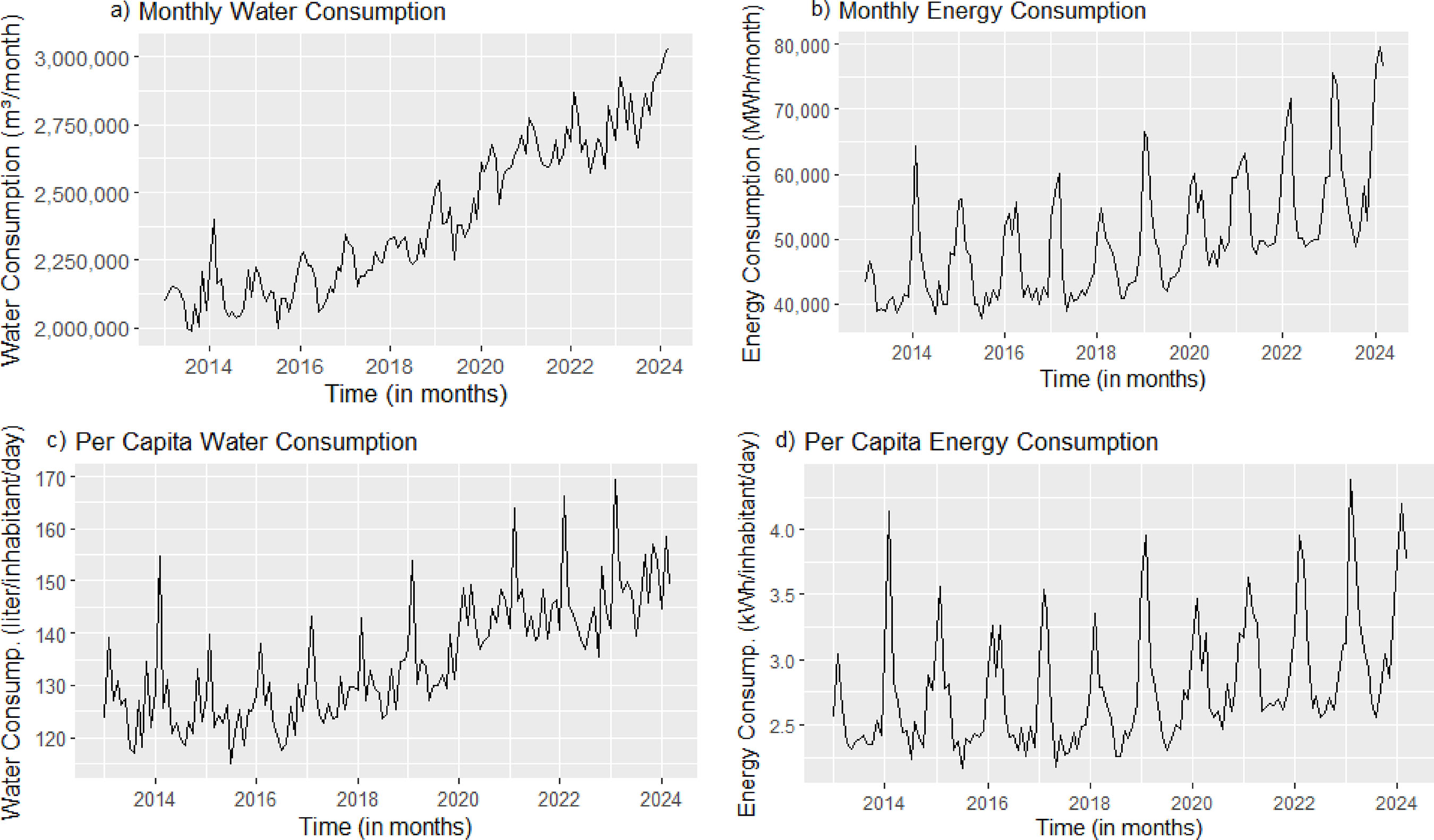
The average monthly water consumption in the city’s residential sector was 2,403,184.34 m³/month, and the average electricity consumption was 49,724.44 MWh/month. The average per capita water consumption during the period was 134.75 liters/inhabitant/day, varying between 114.87 and 169.54 liters/inhabitant/day (in July 2015 and February 2023, respectively). The average per capita electricity consumption was 2.79 kWh/inhabitant/day, with a minimum value of 2.16 kWh/inhabitant/day in July 2015 and a maximum value of 4.39 kWh/inhabitant/day in February 2023. The months and years with the minimum and maximum values of per capita water and electricity consumption are observed to be the same. Regarding total monthly water and energy consumption in the residential sector, the highest values are observed at the end of the series, in February 2024 for electricity (79,689.33 MWh/month) and in March 2024 for water consumption (3,030,607 m³/month).

The analysis of the correlation between monthly water and electricity consumption in the residential sector of the city resulted in a Pearson correlation coefficient $r$ = 0.77 (p-value < 0.01). In the case of per capita consumption, the Pearson correlation coefficient obtained was $r$ = 0.74 (p-value < 0.01). The Spearman correlation coefficients obtained for the total and per capita consumption data were 0.80 and 0.75, respectively, both statistically significant. These values indicate a moderate to strong and significant positive correlation. In the study by Yu et al. (2018), the correlation coefficient between total water and electricity consumption in urban households was 0.60. In the specific case of water and electricity use for activities related to cleaning, cooking and bathing, the coefficient obtained was 0.80. In the work by Chen et al. (2016), the coefficient between domestic energy and water consumption was 0.81 for the city of Beijing and 0.97 for Shanghai. These studies also point to a moderate to strong correlation between water and electricity consumption, as found in this work.

3.2 Time series analysis

Figure 3 presents the time series graphs of total water and electricity consumption in the residential sector of the city of Joinville, in addition to the time series of per capita consumption. Seasonality can be observed, especially in the time series of electricity consumption (Figures 3b and 3d), with an increased consumption in the warmer months of each year. Table 2 presents the results of the ETS and the SARIMA models, as well as metrics for the training and test samples.

Figure 3
Time series graphs: (a) total water consumption in m³/month, (b) total electricity consumption in MWh/month, (c) water consumption per capita in liters/inhabitant/day, (d) electricity consumption per capita in kWh/inhabitant/day

Table 2
ETS and SARIMA models, accuracy metrics for training and test samples, and coefficient of determination between predicted and real values

Model	Data	Unit	RMSE	MAPE	R²
ETS (M,A,A)	Water	m³/month	53,881.67a 82,077.37b	1.92 a 2.39b	0.93 a 0.81 b
ETS (M,Ad,M)	Energy	MWh/month	3,119.62 b 4,054.74b	4.65 a 5.27b	0.76 a 0.82 b
ETS (M,N,A)	Water	L/inhabitant/day	3.33 a 4.06b	2.04a 2.41b	0.89 a 0.62 b
ETS (M,N,M)	Energy	kWh/inhabitant/day	0.18a 0.22b	4.63 a 5.36b	0.82 a 0.83 b
SARIMA (0,1,1)(0,1,1)12	Water	m³/month	56,622.15a 74,660.52b	1.86a 2.33b	0.94 a 0.79 b
SARIMA (0,0,1)(0,1,1)12	Energy	MWh/ month	3,239.10a 4,555.54b	4.61a 4.93b	0.82 a 0.85 b
SARIMA (0,1,1)(0,1,2)12	Water	L/inhabitant/day	3.45a 4.76b	2.01a 2.92b	0.89 a 0.71 b
SARIMA (0,0,1)(2,1,0)12	Energy	kWh/inhabitant/day	0.21a 0.23b	5.16a 4.76b	0.82 a 0.83 b

• Note:
• ^a
  training; and
• ^b
  test.

The analysis of the metrics shows that observed and predicted values are close, especially for SARIMA models. The R² between predicted and real values, close to 1.0, indicates that the series have a good fit and a low training error (James et al., 2021). The SARIMA models exhibit similar but slightly lower MAPE error values for water consumption than the ETS models in this case study. For the SARIMA models, MAPE values between 1.92% and 2.92% show that the predictions have a low percentage of errors, while RMSE values indicate that the average errors of the models, in absolute terms, are low, confirming the high accuracy of the predictions. For electricity consumption, the error values are also similar, with the SARIMA models showing better results for the test data. The SARIMA models show lower values of RMSE and MAPE than simple models, like seasonal naïve. Seasonal naïve present RMSE = 143,930.30 and MAPE = 4.01% for total water consumption and RMSE = 5.47 and MAPE = 3.08% for per capita water consumption. The seasonal naïve models present RMSE = 5,991.7 and MAPE = 7.08% for total electricity consumption and RMSE = 0.25 and MAPE = 5.57% for per capita electricity consumption. Figure 4 presents the time series with prediction estimated values and confidence intervals.

In the forecast of total water consumption in the city’s residential sector (Figure 4a), an exponential smoothing model ETS (M,A,A) with multiplicative error, with additive trend and seasonality, was obtained. The total electricity consumption model obtained (Figure 4b) was ETS (M,Ad,M), with multiplicative error, damped additive trend and multiplicative seasonality. For per capita water consumption (Figure 4c), an ETS (M,N,A) model with multiplicative error, no trend and additive seasonality, was obtained. For per capita electricity consumption (Figure 4d), an ETS (M,N,M) model was obtained, with multiplicative error, no trend and multiplicative seasonality. The seasonality is similar in all series, with increased consumption in the warmer months.

Figure 4
Time series graphs with forecasts: (a) water in m³/month (ETS), (b) electricity in MWh/month (ETS), (c) water in liters/inhabitant/day (ETS), (d) electricity in kWh/inhabitant/day (ETS), (e) water in m³/month (SARIMA), (f) electricity in MWh/month (SARIMA), (g) water in liters/inhabitant/day (SARIMA), (h) electricity in kWh/inhabitant/day (SARIMA)

The multiplicative error in the ETS models is proportional to the forecast and depends on the series’ magnitude, whereas the additive trend and seasonality increase or decrease steadily (Svetunkov, 2023). The damped trend indicates a gradual slowdown in the growth of the series (Svetunkov, 2023), while the multiplicative seasonality indicates a pattern in which the magnitude of fluctuations increases proportionally with the trend (Hyndman; Athanasopoulos, 2021).

In addition to the exponentially smoothed models, analyses were performed using the ARIMA method and seasonal ARIMA models were generated. The model obtained for the total water consumption series in the city’s residential sector (Figure 4e) and for per capita water consumption (Figure 4g) was the SARIMA (0,1,1) (0,1,1)₁₂ and SARIMA (0,1,1) (0,1,2)₁₂ respectively. The regular and seasonal parts do not contain autoregressive components, presenting differentiation to make the series stationary, and a moving average term for better adjustments to the forecasts. The series has trend and seasonality (Hyndman; Athanasopoulos, 2021).

In the case of total electricity consumption in the city’s residential sector (Figure 4f) and per capita consumption (Figure 4h), the models were the SARIMA (0,0,1) (0,1,1)₁₂ (with drift) and the SARIMA (0,0,1) (2,1,0)₁₂ (with drift), respectively. In the seasonal part, the differentiation makes the seasonal series stationary and with drift, indicating that the series has a slight fluctuation in the average growth (Hyndman; Athanasopoulos, 2021). These results show that the electricity consumption series in the city did not grow as much as the water consumption series. The SARIMA forecasting models for total and per capita water consumption showed residuals with no serial dependence, with p-values of 0.57 and 0.84, respectively (Ljung-Box test). The residuals also showed a normal distribution (Jarque-Bera test), with p-values of 0.34 (total water consumption) and 0.43 (per capita water consumption). The residuals of the SARIMA forecasting models for total and per capita electricity consumption did not show a normal distribution (p-value < 0.01). Regarding serial correlation, they presented p-values equal to 0.41 (total electricity consumption) and 0.12 (per capita electricity consumption). Although the forecasting errors for the electricity consumption models are small, obtaining models using other methods is recommended and planned for the continuation of this research work. The results from the residual analysis (Ljung-Box and Jarque-Bera tests) are shown in Table 3.

Table 3
Ljung-Box test for autocorrelation and Jarque-Bera normality test results

Time series	Model	Ljung-Box p-value	Jarque-Bera p-value
Total water consumption	ETS (M,A,A)	0.08	0.61
Per capita water consumption	ETS (M,N,A)	0.24	0.65
Total electricity consumption	ETS (M,Ad,M)	0.07	<0.01
Per capita electricity consumption	ETS (M,N,M)	0.02	<0.01
Total water consumption	SARIMA (0,1,1)(0,1,1)12	0.57	0.34
Per capita water consumption	SARIMA (0,1,1)(0,1,2)12	0.84	0.43
Total electricity consumption	SARIMA (0,0,1)(0,1,1)12	0.41	<0.01
Per capita electricity consumption	SARIMA (0,0,1)(2,1,0)12	0.12	<0.01

The social, political and economic development of nations is closely linked to the use of natural resources (Dias; Mattos; Balestieri, 2006). The results by Dias, Mattos and Balestieri (2006) show that per capita energy consumption increases with the increase in the human development index. Although Joinville’s human development index (HDI) can be considered high (Padilla; Latypov, 2021), in our study, water consumption showed a more pronounced increase than electricity consumption, which may have occurred because Brazilians’ spendings on electricity are considerably higher than on water (Lins; Coelho; Travassos, 2025). Therefore, an increase in water consumption has a proportionally smaller impact on household expenses than an increase in electricity consumption.

This study contributes to the analysis of water and energy consumption patterns in the residential sector of Joinville, in southern Brazil. These results are similar to those found by Ristow et al. (2021) and Estrada, Henning and Kalbusch (2025) for water consumption, with a slight reduction in error metrics. Furthermore, our study includes an analysis of electricity consumption in the city, which has not been fully addressed in recent studies. However, it is important to highlight that classic models such as SARIMA have limitations that models like Prophet could overcome, and that recent advanced machine learning algorithms may produce more accurate results (Salman; Shaka’a, 2026). In this sense, these limitations are also opportunities for continued research.

3.3 Linear regression model

Based on measured residential water and electricity consumption values, two simple linear regression models were fitted (Equations 6 and 7). The first model (Equation 6) will be used to estimate monthly electricity consumption (MWh/month) based on the monthly water consumption predicted by the SARIMA models (in m³/month). The second model (Equation 7) will be used to estimate daily per capita electricity consumption (kWh/inhabitant/day) based on the predicted per capita water consumption (liters/inhabitant/day).

Eq. 6 $y_1=0.02562•x_1-11,852.7$

Where:

$y_1$ is the electricity consumption (MWh/month); and

$x_1$ is the water consumption (m³/month) in the residential sector of the city.

Eq. 7 $y_2=0.03057•x_2-1.331$

Where:

$y_2$ is the per capita electricity consumption (kWh/inhabitant/day); and

$x_2$ is the per capita water consumption (liters/inhabitant/day) in the city.

To forecast electricity consumption, the results of the SARIMA water consumption forecasting models are applied. Using Equation 6, predictions for electricity consumption (in MWh/month) for January, February and March 2024 were calculated, applying to $x_1$ the predicted values for residential water consumption obtained through the SARIMA (0,1,1) (0,1,1)₁₂ model (Figure 4e). The calculated values were compared with the electricity consumption predictions obtained with the SARIMA (0,0,1) (0,1,1)₁₂ model (Figure 4f). The R² between actual and predicted values was R² = 0.99, slightly higher than that obtained with the SARIMA model for the sample (R² = 0.91) for the same forecast period.

Using Equation 7, predictions for per capita electricity consumption for January, February and March 2024 were calculated. The predicted values for per capita water consumption obtained using the SARIMA (0,1,1) (0,1,2)₁₂ model (Figure 4g) were applied to $x_2$. The calculated values were compared with the per capita electricity consumption predictions obtained with the SARIMA (0,0,1) (2,1,0)₁₂ model (Figure 4h). The R² between actual and predicted values was R² = 0.99, slightly higher than that obtained with the SARIMA model for the test sample (R² = 0.97) for the same forecast period. This difference can be explained by the structure of the SARIMA model with drift, which did not capture the damped trend pattern at the end of the series, generating predictions with larger errors. Furthermore, linear regression models circumvent the limitations arising from residual analysis in time series regression for electricity consumption in this study and are an option for future research. Thus, the results show the potential of the proposed modeling with simple linear regression.

3.4 Web application for forecasting water and energy consumption

A web application is being developed to allow the replication of the analyses performed in this manuscript, as well as the use of new data. The application is expected to assist in the integrated analysis of water and electricity consumption in other contexts and locations. To perform the analysis using the application, the data must be loaded in .csv, .xls, or .xlsx format. The columns are available for selection in the time series settings and for linear regression. A screenshot of the application can be seen in Figure 5, and the application can be accessed at Cesconetto, Henning and Kalbusch (2025). Formal validation of the application is part of the ongoing research work.

Figure 5
Screenshot of web application for loading data, analysis types and results

4 Conclusions

This study presented an analysis of time series data on water and energy consumption in the city of Joinville, southern Brazil. Descriptive statistics and correlation analysis provided an initial overview of water and energy consumption in residential buildings in the city. Data corresponding to the total monthly consumption of the city’s residential sector were analyzed, in addition to per capita consumption data. The time series of water and electricity consumption show a strong and significant positive correlation. The analysis of the time series showed seasonal patterns and trends that helped to better understand the behavior of residential water and electricity consumption, suggesting that this approach can be effective for understanding the phenomenon under study and for making predictions. Although the time series for water and electricity consumption show an increasing trend, the growth pattern of water consumption reflects a scenario in which effective actions or policies aimed at reducing water consumption are still needed. Thus, the results from this work provide evidence that there are opportunities for implementing actions focused on efficient water consumption in buildings and urban contexts. The use of simple linear regression using predicted values showed that accurate short-term forecasts can be obtained with less computational effort, which shows the possibility of obtaining accurate forecasts in a more reasonable perspective.

This work has its limitations, including the use of aggregated data and the absense of explanatory variables. As a suggestion for the continuation of this piece of research, the application of time series models with the inclusion of regressor variables and the combination of forecasts from different models is recommended to obtain even more precise results. Furthermore, for the continuity of the work, the application of other approaches, such as the Prophet model and machine learning methods, is suggested for future studies. The integration or combination of predictions is also a research opportunity. Still, studies on water and energy consumption in other sectors, such as industrial, commercial, and public, are also options for future research. The relationship between water and electricity consumption shows the importance of creating public policies with measures to encourage water and electricity conservation practices in an integrated way within the built environment.

Acknowledgements

The authors would like to thank Companhia Águas de Joinville for sharing the water consumption data. This research was supported by Conselho Nacional de Desenvolvimento Científico e Tecnológico (CNPq) and Fundação de Amparo à Pesquisa e Inovação do Estado de Santa Catarina (FAPESC, grants number 2023TR000334 and 2025TR001584).

• CESCONETTO, A. da R.; FLEISCHMANN, L. H.; HENNING, E.; KALBUSCH, A. Predicting residential water and electricity consumption: a case study using time series analysis. Ambiente Construído, Porto Alegre, v. 26, e152285, jan./dez. 2026. ISSN 1678-8621 Associação Nacional de Tecnologia do Ambiente Construído. http://dx.doi.org/10.1590/s1678-86212026000100971
• Financial Support
  This research was supported by Conselho Nacional de Desenvolvimento Científico e Tecnológico (CNPq) and Fundação de Amparo à Pesquisa e Inovação do Estado de Santa Catarina (FAPESC, grants number 2023TR000334 and 2025TR001584).
• Declaration of Generative AI and AI-Assisted Technologies in the Writing Process
  The authors declare that they have not used Generative AI and AI-Assisted Technologies in the writing process of the manuscript.

Data Availability Statement

The water consumption database was provided by Companhia Águas de Joinville and direct requests may apply. Electricity consumption data is available on the website of Centrais Elétricas de Santa Catarina (CELESC, 2024), as stated in section 2.1 of this manuscript. Codes are available from the corresponding author upon reasonable request.

References

• ABDALLAH, A. M.; ROSENBERG, D. E. Heterogeneous residential water and energy linkages and implications for conservation and management. Journal of Water Resources Planning and Management, v. 140, p. 288-297, 2014.
• AGAJ, T. et al. Using ARIMA and ETS models for forecasting water level changes for sustainable environmental management. Scientific Reports, v. 14, p. 22444, 2024.
• AL-CHALABI, H.; AL-DOURI, Y. K.; LUNDBERG, J. Time series forecasting using ARIMA model: a case study of mining face drilling rig. In: INTERNATIONAL CONFERENCE ON ADVANCED ENGINEERING COMPUTING AND APPLICATIONS, 12., Atenas, 2018. Proceedings […] Atenas, Grécia: IARIA, 2018.
• ALMEIDA, A. P.; SOUSA, V.; SILVA, C. M. Methodology for estimating energy and water consumption patterns in university buildings: case study, Federal University of Roraima (UFRR). HELIYON, v. 7, n. 12, p. e08642, 2021.
• CENTRAIS ELÉTRICAS DE SANTA CATARINA. Dados de consumo 2024. Available: https://www.celesc.com.br/home/mercado-de-energia/dados-de-consumo/ Access: 15 jul. 2024.
  » https://www.celesc.com.br/home/mercado-de-energia/dados-de-consumo/
• CESCONETTO, A. R.; HENNING, E.; KALBUSCH, A. Análise de dados e séries temporais 2025. Available: https://yoy02c-aline-cesconetto.shinyapps.io/app-ts/ Access: 02 feb. 2026.
  » https://yoy02c-aline-cesconetto.shinyapps.io/app-ts/
• CHANG, W. et al. Shiny: web application framework for R. R package version 1.8.1.9001. 2024. Available: https://cran.r-project.org/web/packages/shiny/shiny.pdf Access: 02 feb. 2026.
  » https://cran.r-project.org/web/packages/shiny/shiny.pdf
• CHEN, I-C. et al Identifying spatial driving factors of energy and water consumption in the context of urban transformation. Sustainability, v. 13, p. 10503, 2021.
• CHEN, S. et al Interaction relationship between urban domestic energy consumption and water use: a case study of Beijing and Shanghai. Water Policy, v. 18, p. 670-684, 2016.
• CHICCO, D.; WARRENS, M. J.; JURMAN, G. The coefficient of determination R-squared is more informative than SMAPE, MAE, MAPE, MSE and RMSE in regression analysis evaluation. PeerJ Computer Science, v. 7, e623, 2021.
• COMINOLA, A. et al. Segmentation analysis of residential water-electricity demand for customized demand-side management programs. Journal of Cleaner Production, v. 172, p. 1607-1619, 2018.
• DIAS, R. A.; MATTOS, C. R.; BALESTIERI, J. A. P. The limits of human development and the use of energy and natural resources. Energy Policy, v. 34, n. 9, p. 1026-1031, 2006.
• ENBEYLE, W. et al Trend analysis and prediction on water consumption in southwestern Ethiopia. Journal of Nanomaterials, v. 2022, p. 3294954, 2022.
• ESTRADA, A.V.; HENNING, E., KALBUSCH, A. Urban water demand forecasting via artificial neural network models: a case study in Southern Brazil. Discover Sustainability, v. 6, p. 1105, 2025.
• GONZÁLEZ-TORRES, M. et al A review on buildings energy information: trends, end-uses, fuels and drivers. Energy Reports, v. 8, p. 626-637, 2022.
• GUBAREVA, R.; LOPES, R. P. Big Data trends in the analysis of city resources. In: NESMACHNOW, S.; HERNÁNDEZ CALLEJO, L. (ed.). Smart cities ICSC-CITIES 2022. Communications in Computer and Information Science. Cham: Springer, 2023.
• HAVLICEK, L. L.; PETERSON, N. L. Robustness of the Pearson correlation against violations of assumptions. Educational and Psychological Measurement, v. 3, n. 2, p. 373–382, 1976.
• HYNDMAN, R. J. et al A state space framework for automatic forecasting using exponential smoothing methods. International Journal of Forecasting, v. 18, n. 3, p. 439–454, 2002.
• HYNDMAN, R. J. et al Forecasting with exponential smoothing: the state space approach. Berlin: Springer-Verlag, 2008.
• HYNDMAN, R. J.; ATHANASOPOULOS, G. Forecasting: principles and practice. 3. ed. Melbourne: OTexts, 2021.
• HYNDMAN, R. J.; KHANDAKAR, Y. Automatic time series forecasting: the forecast package for R. Journal of Statistical Software, v. 27, n.3, p. 1-22, 2008.
• INSTITUTO BRASILEIRO DE GEOGRAFIA E ESTATÍSTICA. Censo Brasileiro de 2022 2022. Available: https://censo2022.gov.br/panorama/ Access: 17 apr. 2024.
  » https://censo2022.gov.br/panorama/
• JAMES, G. et al An introduction to statistical learning: with applications in R. 2. ed. Cham: Springer, 2021.
• JOINVILLE. Joinville cidade em dados Available: https://www.joinville.sc.gov.br/?post_type=publicacao&s=. Access: 15 feb. 2024.
  » https://www.joinville.sc.gov.br/?post_type=publicacao&s=
• KACHALLA, I. A. et al Data-driven hybrid SARIMAX-MLP framework for energy consumption prediction in residential micro-grid. Results in Engineering, v. 26, p. 105336, 2025.
• KACHALLA, I. A.; GHIAUS, C.; BASEER, M. Comparative analysis of machine learning models for prediction and forecasting of electric water boilers energy consumption. Applied Thermal Engineering, v. 267, p. 125799, 2025.
• KAHRAMAN, E.; AKAY, O. Comparison of exponential smoothing methods in forecasting global prices of main metals. Mineral Economics, v. 36, p. 427–435, 2023.
• LI, Z. et al Enhancing the explanation of household water consumption through the water-energy nexus concept. npj Clean Water, v. 7, n. 8, 2024.
• LINS, J. A. B.; COELHO, A. B.; TRAVASSOS, G. F. The determinants of expenditures with utilities in Brazilian households. Revista Brasileira de Estudos Regionais e Urbanos, v. 19, n. 1, p. 127–149, 2025.
• LIU, M.; FANG, C.; BAI, Y. Exploring the relationship between water–energy consumption and urbanization in China: a urban-rural transformation perspective. Environmental Impact Assessment Review, v. 112, 107834, 2025.
• MATOS, C. et al Water and energy consumption in urban and rural households. In: INTERNATIONAL SYMPOSIUM OF CIB W062 – WATER SUPPLY AND DRAINAGE FOR BUILDINGS, 39., Nagano, 2013. Proceedings […] Nagano: Shinshu University, 2013.
• MONTGOMERY, D. C.; RUNGER, G. C.; HUBELE, N. F. Engineering statistics 5 ed. Hoboken: Wiley, 2011.
• MOORE, D. S. The basic practice of statistics 4. ed. New York: Freeman, 2007.
• MUSTAFA, A. T.; AL-YOZBAKY, O. S. A. D. Forecasting energy demand and generation using time series models: a comparative analysis of classical, grey, fuzzy, and intelligent approaches. Franklin Open, v. 12, p. 100350, 2025.
• NASERI, M. Y. et al Patterns and predictors of residential indoor water use across major US cities. Earth’s Future, v. 13, p. e2024EF005467, 2025.
• PADILLA, M.; LATYPOV, V. The city lab joinville in southern Brazil: an innovative approach for addressing sustainability in the mobility sector. 2021. Available: https://www.iuk.fraunhofer.de/content/dam/iuk/whitepapers/en/iao/2021_IAO_WP_The%20City%20Lab%20Joinville%20in%20southern%20Brazil_EN.pdf Access: 02 feb. 2026.
  » https://www.iuk.fraunhofer.de/content/dam/iuk/whitepapers/en/iao/2021_IAO_WP_The%20City%20Lab%20Joinville%20in%20southern%20Brazil_EN.pdf
• R CORE TEAM. R: a language and environment for statistical computing. Vienna: R Foundation for Statistical Computing, 2025.
• RISTOW, D. C. M. et al for forecasting water demand using time series analysis: a case study in Southern Brazil. Journal of Water, Sanitation and Hygiene for Development, v. 11, n. 2, p. 231–240, 2021.
• SALMAN, A.; SHAKA’A, Y. Automated water demand forecasting for national-scale deployment: a prophet-based framework for Palestinian municipal water management. Scientific Reports, v. 16, p. 3295, 2026.
• SCHOBER, P.; BOER, C.; SCHWARTE, L. A. Correlation coefficients: appropriate use and interpretation. Anesthesia & Analgesia, v. 126, n. 5, p. 1763-1768, 2018.
• SVETUNKOV, I. Forecasting and analytics with the Augmented Dynamic Adaptive Model (ADAM). Boca Raton: Chapman and Hall/CRC, 2023.
• TSAY, R. S. Time series and forecasting: brief history and future research. Journal of the American Statistical Association, v. 95, n. 450, p. 638–43, 2000.
• WANG, D.; ZHANG, Y.; YOUSEFI, N. Urban water-energy consumption prediction influenced by climate change utilizing an innovative deep learning method. Scientific Reports, v.14, p. 30931, 2024.
• YAN, G. et al Water-energy trajectories for urban water and wastewater reveal the impact of city strategies. Applied Energy, v. 366, p. 123292, 2024.
• YU, M. et al Water and related electrical energy use in urban households: influence of individual attributes in Beijing, China. Resources, Conservation & Recycling, v.130, p. 190-199, 2018.
• ZENG, Q. et al Time series analysis of temporal trends in the pertussis incidence in Mainland China from 2005 to 2016. Scientific Reports, v. 6, p. 32367, 2016.

Edited by

• Editor in-chief:
  Enedir Ghisi

Publication Dates

• Publication in this collection
  22 May 2026
• Date of issue
  Jan-Dec 2026

History

• Received
  10 Dec 2025
• Reviewed
  04 Feb 2026
• Accepted
  13 Feb 2026