New vector norms, seminorms and exact solutions as a benchmark for the steady-state convection-diffusion equation

Abstract

The steady-state convection-diffusion equation is part of the mathematical model for transport phenomena. Its exact solution may present boundary layers when convection is dominant. In these cases, numerical solutions of the second-order centered finite difference present spurious oscillations, and stabilized methods may present the smearing effect. Here new $h_1$ and $h_2$ vector norms and seminorms are proposed as analogs to the $H^1$ and $H^2$ norms used in the finite element framework, which allow defining new errors for the solutions and their derivatives obtained by the finite difference method. In addition, new $w{l}_2$, $w{h}_1$ and $w{h}_2$ weighted norms and seminorms are introduced, allowing to observe convergences of the schemes similar to what should be expected theoretically. These norms and seminorms and their weighted versions are valid for uniform and non-uniform meshes. Furthermore, exact solutions with boundary layers are proposed as benchmarks together with the errors in the new vector norms of two classical finite difference schemes: centered and upwind. Numerical results indicate that a mesh that guarantees an acceptable approximation for the solution $u$ does not guarantee an acceptable approximation for the derivatives of $u$. For this reason non-uniform meshes and new schemes will be analyzed in future articles.

Key words
diffusion - advection; finite difference method; vector norms; vector seminorms; exact solutions; stabilization

INTRODUCTION

The steady-state convection-diffusion problem is described by equations (1)-(2).

$$\underset{Diffusion}{\underbrace{-\nabla \cdot \left(D\nabla u\right)}}+\underset{Advection}{\underbrace{v\cdot \nabla u}}=f\mathrm{\text{in}}\Omega ,$$(1)

$$u=g\mathrm{\text{on}}\partial \Omega ,$$(2)

where $\Omega \subset {ℝ}^n(n=1,2)$ is open bounded domain with a Lipschitz boundary $\partial \Omega$, $u$ is the unknown scalar quantity of the problem to be transported by advection and diffusion, $0<D_{min}\le D\le D_{max}$ is the diffusive coefficient whose lower and upper bounds are $D_{min}$ and $D_{max}$, $f\in L^2\left(\Omega \right)$ is a volume source term, $v=(v_1,\dots ,v_n)$ is the transport advective field with $v_i\in H^1\left(\Omega \right)$, $g\in C^0\left(\partial \Omega \right)$ is the boundary value prescribed for $u$, $L^2\left(\Omega \right)$ is the space of square integrable functions on $\Omega$, $H^1\left(\Omega \right)$ is the Hilbert space whose functions and their derivatives are square integrable functions on $\Omega$, and $C^0\left(\partial \Omega \right)$ is the space of continuous functions in $\partial \Omega$. The functions $D:\Omega \to ℝ$, $v_i:\Omega \to ℝ$, $f:\Omega \to ℝ$, $g:\partial \Omega \to ℝ$ are all known data of the problem. This equation is used to model transport phenomena, present in several areas of knowledge. For example, in mechanical engineering there are several applications in fluid mechanics (Raithby 1976, Brooks & Hughes 1982, Galeão & Carmo 1988, Alvarez et al. 2017, Almeida et al. 2018, Bermúdez et al. 2021), and in medicine it is used to model the growth of brain tumors (Rockne et al. 2009, Silva 2014, Jesus et al. 2016, Machado et al. 2023). The Péclet number $P_e=\frac{\left|v\right|L}{D}$ is a dimensionless quantity that estimates the ratio of the rate of advection to the rate of diffusion, where $L$ is a characteristic length, and $|\circ |$ denotes the absolute value of a vector or scalar. In cases where $P_e<1$ diffusion is said to be dominant, and the exact solution does not have large gradients. When $P_e>1$ convection is said to be dominant, and the exact solution may have boundary layers. Boundary layers are small subregions of $\Omega$ where derivatives of the solution are very large.

It is well known that numerical solutions by classical finite difference (FDM), finite element (FEM) and finite volume (FVM) methods are accurate and stable when diffusion is dominant. However, when convection is dominant, these numerical solutions lose stability and may present spurious oscillations in the presence of boundary layers (Stynes & Stynes 2018). This led to the emergence of so-called stabilized formulations, which present greater stability than classical formulations in the presence of boundary layers (Courant et al. 1952, Raithby 1976, Brooks & Hughes 1982, Galeão & Carmo 1988, Carmo & Alvarez 2003, 2004). However, some of these stabilized formulations may present the so-called smearing effect, which results in an excessive smoothing of the numerical solution that appears both in regions with boundary layers and in regions where the exact solution is smooth. Therefore, whenever a new stabilized formulation is developed, it is necessary to evaluate its performance in terms of accuracy and stability, where two important aspects to be evaluated are the elimination of spurious oscillations and the reduction of the smearing effect. These two aspects are considered to be the two main ‘pathologies’ that numerical methods present.

There are a set of model problems or test problems that are used as benchmarks to verify the performance of stabilized methods. Most of these model problems are cases where the exact solution should be smooth or have boundary layers. However, there are few known exact solutions with boundary layers. Generally, only the shape of the solution is known, but without the exact formulas. Knowing the formulas of the exact solutions is important because it allows the a posteriori error to be calculated, and thus a more quantitative than qualitative study of the error of the numerical method can be performed. In addition, cases with known exact solutions allow the calculation of the error for the derivatives of the numerical solution, as will be presented in the next section.

Exact solutions of the convection-diffusion equation have been a topic of research that continues to be current for mathematicians, physicists and engineers (Ivanova 2008, Portegies & Duits 2017). However, this type of approach is not the focus of this paper. Here the focus is on cases that have smooth exact solutions and boundary layers to study the performance of the numerical methods. Therefore, some exact solutions that have a shape very similar to that of the model problems used as benchmarks are presented, as well as the errors for the solution and their derivatives of two classical finite difference schemes: centered and upwind. On the other hand, exact solutions, in addition to being important elements in the analysis of the performance of numerical methods, contribute to the verification and validation of computational codes.

The finite difference method is the oldest numerical method for solving Partial Differential Equation (PDE), and it has some disadvantages when compared to FEM. One of these disadvantages is that it only has the Euclidean norm in its framework. Different norms and seminorms are important tools in the analysis of numerical methods, since they allow the evaluation of the contribution of the solution and its derivatives to the error. In the finite element framework, the $L^2\left(\Omega \right)$, $H^1\left(\Omega \right)$ and $H^2\left(\Omega \right)$ norms and seminorms are frequently used. Here, for the first time, new $h_1$ and $h_2$ norms and seminorms analogous to $H^1\left(\Omega \right)$ and $H^2\left(\Omega \right)$ norms and seminorms are introduced. In addition, two versions of the Euclidean norm are presented: the traditional Euclidean vector norm ($l_2$), and a version called the weighted norm ($w{l}_2$) (Alvarez et al. 2025). These two versions are also extended to the $h_1$ and $h_2$ norms and seminorms. In this way, it is possible to define new global errors for the solutions and their derivatives obtained by the finite difference method.

In essence, this work presents two new contributions to the analysis of finite difference schemes. The first novelty consists of the introduction of new norms and semi-norms in the finite difference framework. The second new feature concerns exact solutions with boundary layers as benchmarks together with the errors in the new vector norms. Among the exact solutions presented, the solutions to model problems with external and internal boundary layers for the 2D case stand out. As far as the authors know, these two solutions are unpublished, and they allow for a quantitative analysis of the errors. The rest of the paper is organized as follows. In the next section, the norms, seminorms and errors are introduced for two classical finite difference schemes. Subsequently, the cases with exact solutions proposed as benchmarks are presented and analyzed, culminating with the conclusions.

MATERIALS AND METHODS

Two computer software were used in this work. Mathematica software (Wolfram 2015) (https://www.wolfram.com/mathematica) was used to perform some symbolic calculations. The MATLAB software (Gilat 2014) (https://www.mathworks.com/products/matlab.html) was used to develop two computational codes, which allowed obtaining the numerical results.

New $h_1$, $h_2$, $w{l}_2$, $w{h}_1$ and $w{h}_2$ vector norms and seminorms were proposed. One-dimensional and two-dimensional cases with exact solution were introduced and compared with the numerical solutions of two finite difference schemes. The global error of each scheme was calculated for the $l_2$, $w{l}_2$, $h_1$, $w{h}_1$, $h_2$, $w{h}_2$ norms and $h_1$, $w{h}_1$, $h_2$, $w{h}_2$ seminorms.

Before starting the theoretical development, it is necessary to clarify the definitions of norm and seminorm (Lebedev et al. 2002, Adams & Fournier 2003). Thus, consider a linear vector space $S$ whose generic elements are denoted by $\phi$. A norm $\parallel \phi {\parallel }_m$ is defined in the space $S$ if the real valued function $\parallel \circ {\parallel }_m\to ℝ$ satisfies the following three properties:

• $\parallel \phi +\varphi {\parallel }_m\le \parallel \phi {\parallel }_m+\parallel \varphi {\parallel }_m$ for all $\phi ,\varphi \in S$,

• $\parallel \lambda \phi {\parallel }_m=\left|\lambda \right|\parallel \phi {\parallel }_m$ for all $\phi \in S$ and all scalars $\lambda$,

• $\parallel \phi {\parallel }_m\ge 0$ for all $\phi \in S$, and $\parallel \phi {\parallel }_m=0$ if and only if $\phi =0$.

A seminorm ${\left|\phi \right|}_m$ is defined in space $S$ if the real valued function ${|\circ |}_m\to ℝ$ satisfies the following three properties:

• ${|\phi +\varphi |}_m\le {\left|\phi \right|}_m+{\left|\varphi \right|}_m$ for all $\phi ,\varphi \in S$,

• ${\left|\lambda \phi \right|}_m=\left|\lambda \right|{\left|\phi \right|}_m$ for all $\phi \in S$ and all scalars $\lambda$,

• ${\left|\phi \right|}_m\ge 0$ for all $\phi \in S$, and ${\left|\phi \right|}_m=0$ if $\phi =0$.

New vector norms, seminorms and errors for finite difference method

In functional analysis there are the well-known $L^2\left(\Omega \right)$, $H^1\left(\Omega \right)$ and $H^2\left(\Omega \right)$ norms (Lebedev et al. 2002, Adams & Fournier 2003, Evans 2010). These norms are used to estimate the error of the solution and derivatives obtained by the finite element method (Brooks & Hughes 1982, Galeão & Carmo 1988, Carmo & Alvarez 2003). The Euclidean vector norm, also known as $l_2$ norm, is the analogue of the $L^2\left(\Omega \right)$ norm. However, as far as the authors know, there is no vector norm analogous to the standard function space $H^1\left(\Omega \right)$ and $H^2\left(\Omega \right)$ norms. Here, the $h_1$ and $h_2$ vector norms are suggested as the analogues of $H^1\left(\Omega \right)$ and $H^2\left(\Omega \right)$ norms. These new norms allow defining new errors for the solutions and their derivatives obtained by the finite difference method.

The analysis is performed for two finite difference schemes in one-dimensional (1D) and two-dimensional (2D) cases, which are representative of the two ‘pathologies’ described in the Introduction: spurious oscillations and the smearing effect. Second-order centered finite difference presents spurious oscillations (numerical instability) in the presence of boundary layers when convection is dominant. Upwind finite difference eliminates spurious oscillations (numerical stability) in the presence of boundary layers when convection is dominant, but has the smearing effect.

1D case and 3-point stencil

In this case $\Omega =]a,b[$, and the standard function space $L^2\left(\Omega \right)$, $H^1\left(\Omega \right)$ and $H^2\left(\Omega \right)$ norms are defined by the equations (3), (4) and (5), where $|\circ |$ denotes the absolute value of a function or a vector (Lebedev et al. 2002, Adams & Fournier 2003, Evans 2010).

$$\parallel u{\parallel }_{L^2\left(\Omega \right)}:={\left({\int }_a^b{\left|u\right|}^{2}dx\right)}^{\frac{1}{2}}.$$(3)

$$\parallel u{\parallel }_{H^1\left(\Omega \right)}:={\left({\int }_a^b[{\left|u\right|}^2+{\left|\frac{du}{dx}\right|}^2]dx\right)}^{\frac{1}{2}}.$$(4)

$$\parallel u{\parallel }_{H^2\left(\Omega \right)}:={\left({\int }_a^b[{\left|u\right|}^2+{\left|\frac{du}{dx}\right|}^2+{\left|\frac{d^{2}u}{d{x}^2}\right|}^2]dx\right)}^{\frac{1}{2}}.$$(5)

These norms are defined in an infinite-dimensional space, with $u$ being the exact solution of equation (1). The Euclidean vector norm $\parallel U{\parallel }_{l_2}$ is the analogue of the $L^2\left(\Omega \right)$ norm for the numerical solution vector $U$ obtained by the finite difference method.

$$\parallel U{\parallel }_{l_2}:={\left(\sum _{i=1}^{N_x}{\left|U_i\right|}^2\right)}^{\frac{1}{2}},$$(6)

where $U_i$ is the value of the approximated solution at grid point $x_i$, and $N_x$ is the dimension of the vector $U$. Therefore, this norm is defined in a finite-dimensional space. However, there is no vector norm for the numerical solution $U$ analogous to the $H^1\left(\Omega \right)$ and $H^2\left(\Omega \right)$ norms. Here, the $h_1$ and $h_2$ norms are suggested for a finite-dimensional vector space:

$$\parallel U{\parallel }_{h_1}:={\left(\sum _{i=1}^{N_x}[{\left|U_i\right|}^2+{\left|U_i^{\left(1\right)}\right|}^2]\right)}^{\frac{1}{2}},$$(7)

$$\parallel U{\parallel }_{h_2}:={\left(\sum _{i=1}^{N_x}[{\left|U_i\right|}^2+{\left|U_i^{\left(1\right)}\right|}^2+{\left|U_i^{\left(2\right)}\right|}^2]\right)}^{\frac{1}{2}},$$(8)

where $U_i^{\left(1\right)}\approx \frac{du\left(x_i\right)}{dx}$ and $U_i^{\left(2\right)}\approx \frac{d^{2}u\left(x_i\right)}{d{x}^2}$ are the approximate derivatives by consistent finite difference formulas. For example, equations (10) and (11) define the formulas for $U_i^{\left(1\right)}$ and $U_i^{\left(2\right)}$ in the classical centered scheme.

Thus, consider a uniform grids and 3-point stencil, the generic equation for the central node $i$ of the stencil is

$$A{U}_{i-1}+B{U}_i+C{U}_{i+1}=f_i,$$(9)

where $U_{i-1}=U(x_i-h)$, $U_i=U\left(x_i\right)$, $U_{i+1}=U(x_i+h)$ and $h=\Delta x$. The derivatives in the equation (1) are approximated as follows (LeVeque 2007). Equation (10) is the traditional second-order accuracy formula for $\frac{d^{2}u}{d{x}^2}$.

$$\frac{d^{2}u\left(x_i\right)}{d{x}^2}\approx U_i^{\left(2\right)}:=\frac{U_{i-1}-2U_i+U_{i+1}}{h^2}.$$(10)

In the classical centered finite difference scheme (CC)

$$\frac{du\left(x_i\right)}{dx}\approx U_{i,CC}^{\left(1\right)}:=\frac{-U_{i-1}+U_{i+1}}{2h},$$(11)

then $A=\frac{-D}{h^2}-\frac{v}{2h}$, $B=\frac{2D}{h^2}$ and $C=\frac{-D}{h^2}+\frac{v}{2h}$. On the other hand, for the upwind finite difference scheme (UPW) (Courant et al. 1952)

$$\frac{du\left(x_i\right)}{dx}\approx U_{i,UPW}^{\left(1\right)}:=\{\begin{array}{cc}\frac{-U_{i-1}+U_i}{h}\hfill & \mathrm{\text{if}}v>0\hfill \\ \frac{-U_i+U_{i+1}}{h}\hfill & \mathrm{\text{if}}v<0\hfill \end{array},$$(12)

then

$$\{\begin{array}{cc}A=\frac{-D}{h^2}-\frac{v}{h},B=\frac{2D}{h^2}+\frac{v}{h},C=\frac{-D}{h^2}\hfill & \mathrm{\text{if}}v>0\hfill \\ A=\frac{-D}{h^2},B=\frac{2D}{h^2}-\frac{v}{h},C=\frac{-D}{h^2}+\frac{v}{h}\hfill & \mathrm{\text{if}}v>0\hfill \end{array}.$$(13)

The local truncation error $\tau$ is obtained by substituting the exact solution $u$ into equation (9) for each scheme (LeVeque 2007). Thus, using the notation $u_i^{\left(n\right)}=\frac{d^{n}u\left(x_i\right)}{d{x}^n}$ the $\tau$ for each scheme are obtained.

$$\mathbf{\text{𝐂𝐂:}}{\tau }_i=(v{u}_i^{\left(3\right)}-\frac{D}{2}{u}_i^{\left(4\right)})\frac{h^2}{6}+𝒪\left(h^3\right).$$(14)

$$\mathbf{\text{𝐔𝐏𝐖:}}{\tau }_i=\{\begin{array}{cc}-\frac{v{u}_i^{\left(2\right)}}{2}h+𝒪\left(h^2\right)\hfill & \mathrm{\text{if}}v>0\hfill \\ \frac{v{u}_i^{\left(2\right)}}{2}h+𝒪\left(h^2\right)\hfill & \mathrm{\text{if}}v>0\hfill \end{array}.$$(15)

The error of the numerical solution at each node $i$ is defined as $\Delta U_i=U_i-u_i$ , the error of the first derivative as $\Delta U_i^{\left(1\right)}=U_i^{\left(1\right)}-u_i^{\left(1\right)}$, and the error of the second derivative as $\Delta U_i^{\left(2\right)}=U_i^{\left(2\right)}-u_i^{\left(2\right)}$, where $U_i^{\left(1\right)}$ is calculated using equations (11) or (12), and $U^{\left(2\right)}$ is calculated using equation (10). The global error of the solution and its derivatives is denoted by $\parallel E^{GU}{\parallel }_m$, $\parallel E^{G{U}^{\left(1\right)}}{\parallel }_m$ and $\parallel E^{G{U}^{\left(2\right)}}{\parallel }_m$, where $\parallel \circ {\parallel }_m$ denotes some vector norm.

Two versions of the Euclidean norm are used here. Equation (16) is the traditional Euclidean vector norm. Equation (17) is a version proposed in the context of rectangular matrices, and can be understood as mean values when compared to the $l_2$ (Alvarez et al. 2025). For this reason it was called a weighted norm $\parallel \circ {\parallel }_{wm}$. Weighted norms were suggested in Alvarez et al. (2025) because using traditional matrix norms (Euclidean, Maximum absolute column sum, Maximum absolute row sum, Frobenius) to perform sensitivity analysis (Alvarez et al. 2021, de Almeida et al. 2021), the theoretical upper bounds for the error were always greatly overestimated.

$$\parallel E^{GU}{\parallel }_{l_2}:={\left(\sum _{i=1}^{N_x}{\left|\Delta U_i\right|}^2\right)}^{\frac{1}{2}}.$$(16)

$$\parallel E^{GU}{\parallel }_{w{l}_2}:=\frac{1}{N_x}{\left(\sum _{i=1}^{N_x}{\left|\Delta U_i\right|}^2\right)}^{\frac{1}{2}}=\frac{\parallel E^{GU}{\parallel }_{l_2}}{N_x}.$$(17)

It should be noted that the weighted norm does not depend on the mesh shape, i.e., equation (17) is valid for both uniform and non-uniform meshes. Furthermore, these two versions of the Euclidean norm are equivalent, since they are defined in a finite-dimensional vector space. The geometric interpretation of both versions of the Euclidean norm is straightforward. The traditional norm corresponds to the Euclidean length of a vector $U$ in the $N_x$-dimensional real vector space ${ℝ}^{N_x}$. The weighted norm corresponds to the average length of the components of the vector $U$ in ${ℝ}^{N_x}$.

Thus, considering the errors $\Delta U_i^{\left(1\right)}$, $\Delta U_i^{\left(2\right)}$ and the new $h_1$ and $h_2$ norms defined previously, it is also possible to measure the global error in the following new norms.

$$\parallel E^{GU}{\parallel }_{h_1}:={\left(\sum _{i=1}^{N_x}[{\left|\Delta U_i\right|}^2+{\left|\Delta U_i^{\left(1\right)}\right|}^2]\right)}^{\frac{1}{2}}.$$(18)

$$\parallel E^{GU}{\parallel }_{w{h}_1}:=\frac{1}{N_x}{\left(\sum _{i=1}^{N_x}[{\left|\Delta U_i\right|}^2+{\left|\Delta U_i^{\left(1\right)}\right|}^2]\right)}^{\frac{1}{2}}.$$(19)

$$\parallel E^{GU}{\parallel }_{h_2}:={\left(\sum _{i=1}^{N_x}[{\left|\Delta U_i\right|}^2+{\left|\Delta U_i^{\left(1\right)}\right|}^2+{\left|\Delta U_i^{\left(2\right)}\right|}^2]\right)}^{\frac{1}{2}}.$$(20)

$$\parallel E^{GU}{\parallel }_{w{h}_2}:=\frac{1}{N_x}{\left(\sum _{i=1}^{N_x}[{\left|\Delta U_i\right|}^2+{\left|\Delta U_i^{\left(1\right)}\right|}^2+{\left|\Delta U_i^{\left(2\right)}\right|}^2]\right)}^{\frac{1}{2}}.$$(21)

2D case and 5-point stencil

In this case, the standard function space $L^2\left(\Omega \right)$, $H^1\left(\Omega \right)$ and $H^2\left(\Omega \right)$ norms are defined by the equations (22), (23) and (24) (Lebedev et al. 2002, Adams & Fournier 2003, Evans 2010).

$$\parallel u{\parallel }_{L^2\left(\Omega \right)}:={\left({\int }_{\Omega }{\left|u\right|}^{2}dxdy\right)}^{\frac{1}{2}}.$$(22)

$$\parallel u{\parallel }_{H^1\left(\Omega \right)}:={\left({\int }_{\Omega }[{\left|u\right|}^2+{\left|\frac{\partial u}{\partial x}\right|}^2+{\left|\frac{\partial u}{\partial y}\right|}^2]dxdy\right)}^{\frac{1}{2}}.$$(23)

$$\parallel u{\parallel }_{H^2\left(\Omega \right)}:={\left({\int }_{\Omega }[{\left|u\right|}^2+{\left|\frac{\partial u}{\partial x}\right|}^2+{\left|\frac{\partial u}{\partial y}\right|}^2+{\left|\frac{{\partial }^{2}u}{\partial x^2}\right|}^2+{\left|\frac{{\partial }^{2}u}{\partial y^2}\right|}^2+2{\left|\frac{{\partial }^{2}u}{\partial x\partial y}\right|}^2]dxdy\right)}^{\frac{1}{2}}.$$(24)

Again, the Euclidean vector norm $\parallel U{\parallel }_{l_2}$ is the analogue of the $L^2\left(\Omega \right)$ norm for the numerical solution vector obtained by the finite difference method.

$$\parallel U{\parallel }_{l_2}:={\left(\sum _{i,j=1}^{N_x,N_y}{\left|U_{i,j}\right|}^2\right)}^{\frac{1}{2}},$$(25)

where $U_{i,j}$ is the value of the approximated solution at grid point $(x_i,y_j)$, and $N_x{N}_y$ is the dimension of the vector $U$. Now, the new $h_1$ and $h_2$ norms are suggested:

$$\parallel U{\parallel }_{h_1}:={\left(\sum _{i,j=1}^{N_x,N_y}[{\left|U_{i,j}\right|}^2+{\left|U_{i,j}^{\left(1x\right)}\right|}^2+{\left|U_{i,j}^{\left(1y\right)}\right|}^2]\right)}^{\frac{1}{2}},$$(26)

$$\parallel U{\parallel }_{h_2}:={\left(\sum _{i,j=1}^{N_x,N_y}[{\left|U_{i,j}\right|}^2+{\left|U_{i,j}^{\left(1x\right)}\right|}^2+{\left|U_{i,j}^{\left(1y\right)}\right|}^2+{\left|U_{i,j}^{\left(2x\right)}\right|}^2+{\left|U_{i,j}^{\left(2y\right)}\right|}^2+2{\left|U_{i,j}^{\left(1x1y\right)}\right|}^2]\right)}^{\frac{1}{2}},$$(27)

where $U_{i,j}^{\left(1x\right)}\approx \frac{\partial u(x_i,y_j)}{\partial x}$, $U_{i,j}^{\left(1y\right)}\approx \frac{\partial u(x_i,y_j)}{\partial y}$, $U_{i,j}^{\left(2x\right)}\approx \frac{{\partial }^{2}u(x_i,y_j)}{\partial x^2}$, $U_{i,j}^{\left(2y\right)}\approx \frac{{\partial }^{2}u(x_i,y_j)}{\partial y^2}$ and $U_{i,j}^{\left(1x1y\right)}\approx \frac{{\partial }^{2}u(x_i,y_j)}{\partial x\partial y}$ are the approximate derivatives by consistent finite difference formulas. Thus, consider a uniform grids and 5-point stencil, the generic equation for the central node $i,j$ of the stencil is

$$A_1{U}_{i,j-1}+A_2{U}_{i-1,j}+B{U}_{i,j}+C_1{U}_{i+1,j}+C_2{U}_{i,j+1}=f_{i,j}.$$(28)

The derivatives in the equation (1) are approximated as follows (LeVeque 2007).

$$\frac{{\partial }^{2}u(x_i,y_j)}{\partial x^2}\approx U_{i,j}^{\left(2x\right)}:=\frac{U_{i-1,j}-2U_{i,j}+U_{i+1,j}}{h^2}.$$(29)

$$\frac{{\partial }^{2}u(x_i,y_j)}{\partial y^2}\approx U_{i,j}^{\left(2y\right)}:=\frac{U_{i,j-1}-2U_{i,j}+U_{i,j+1}}{h^2}.$$(30)

In the classical centered scheme

$$\frac{\partial u(x_i,y_j)}{\partial x}\approx U_{i,j,CC}^{\left(1x\right)}:=\frac{-U_{i-1,j}+U_{i+1,j}}{2h},$$(31)

$$\frac{\partial u(x_i,y_j)}{\partial y}\approx U_{i,j,CC}^{\left(1y\right)}:=\frac{-U_{i,j-1}+U_{i,j+1}}{2h},$$(32)

then $A_1=-\frac{D}{h^2}-\frac{v_2}{2h}$, $A_2=-\frac{D}{h^2}-\frac{v_1}{2h}$, $B=\frac{2D}{h^2}+\frac{2D}{h^2}$, $C_1=-\frac{D}{h^2}+\frac{v_1}{2h}$ and $C_2=-\frac{D}{h^2}+\frac{v_2}{2h}$. On the other hand, for the upwind scheme

$$\frac{\partial u(x_i,y_j)}{\partial x}\approx U_{i,j,UPW}^{\left(1x\right)}:=\{\begin{array}{cc}\frac{-U_{i-1,j}+U_{i,j}}{h}\hfill & \mathrm{\text{if}}{v}_1>0\hfill \\ \frac{-U_{i,j}+U_{i+1,j}}{h}\hfill & \mathrm{\text{if}}{v}_1>0\hfill \end{array},$$(33)

$$\frac{\partial u(x_i,y_j)}{\partial y}\approx U_{i,j,UPW}^{\left(1y\right)}:=\{\begin{array}{cc}\frac{-U_{i,j-1}+U_{i,j}}{h}\hfill & \mathrm{\text{if}}{v}_2>0\hfill \\ \frac{-U_{i,j}+U_{i,j+1}}{h}\hfill & \mathrm{\text{if}}{v}_2>0\hfill \end{array},$$(34)

and depending on the sign of $v_1$ and $v_2$, four possibilities arise. If $v_1\ge 0$ and $v_2>0$, then $A_1=-\hat{A}-\widehat{C_y}$, $A_2=-\hat{A}-\widehat{C_x}$, $B=4\hat{A}+\widehat{C_x}+\widehat{C_y}$ and $C_1=C_2=-\hat{A}$, where $\hat{A}=\frac{D}{h^2}$, $\widehat{C_x}=\frac{v_1}{h}$ and $\widehat{C_y}=\frac{v_2}{h}$. If $v_1>0$ and $v_2\ge 0$, then $A_1=-\hat{A}-\widehat{C_y}$, $A_2=-\hat{A}$, $B=4\hat{A}-\widehat{C_x}+\widehat{C_y}$, $C_1=-\hat{A}+\widehat{C_x}$ and $C_2=-\hat{A}$. If $v_1>0$ and $v_2\le 0$, then $A_1=-\hat{A}$, $A_2=-\hat{A}-\widehat{C_x}$, $B=4\hat{A}+\widehat{C_x}-\widehat{C_y}$, $C_1=-\hat{A}$ and $C_2=-\hat{A}+\widehat{C_y}$. If $v_1\le 0$ and $v_2>0$, then $A_1=A_2=-\hat{A}$, $B=4\hat{A}-\widehat{C_x}-\widehat{C_y}$, $C_1=-\hat{A}+\widehat{C_x}$ and $C_2=-\hat{A}+\widehat{C_y}$. If $v_1=0$, then $\widehat{C_x}=0$ and the case according to the sign of $v_2$ should be chosen. Similarly, if $v_2=0$, then $\widehat{C_y}=0$ and the case according to the sign of $v_1$ should be chosen.

Using the notation $u_{i,j}^{\left(nx\right)}=\frac{{\partial }^{n}u(x_i,y_j)}{\partial x^n}$ and $u_{i,j}^{\left(ny\right)}=\frac{{\partial }^{n}u(x_i,y_j)}{\partial y^n}$, the local truncation error is obtained for each scheme.

$$\mathbf{\text{𝐂𝐂:}}{\tau }_{i,j}=[v_1{u}_{i,j}^{\left(3x\right)}+v_2{u}_{i,j}^{\left(3y\right)}-\frac{D}{2}(u_{i,j}^{\left(4x\right)}+u_{i,j}^{\left(4y\right)})]\frac{h^2}{6}+𝒪\left(h^3\right).$$(35)

$$\mathbf{\text{𝐔𝐏𝐖:}}{\tau }_{i,j}=[\mp v_1{u}_{i,j}^{\left(2x\right)}\mp v_2{u}_{i,j}^{\left(2y\right)}]h+[v_1{u}_{i,j}^{\left(3x\right)}+v_2{u}_{i,j}^{\left(3y\right)}]\frac{h^2}{6}+𝒪\left(h^3\right),$$(36)

where the sign $-$ or $+$ in $\mp$ depends on the sign of $v_1$ and $v_2$.

Similarly to the 1D case, the errors at each node $i,j$ are calculated as $\Delta U_{i,j}=U_{i,j}-u_{i,j}$, $\Delta U_{i,j}^{\left(1x\right)}=U_{i,j}^{\left(1x\right)}-u_{i,j}^{\left(1x\right)}$, $\Delta U_{i,j}^{\left(1y\right)}=U_{i,j}^{\left(1y\right)}-u_{i,j}^{\left(1y\right)}$, $\Delta U_{i,j}^{\left(2x\right)}=U_{i,j}^{\left(2x\right)}-u_{i,j}^{\left(2x\right)}$, $\Delta U_{i,j}^{\left(2y\right)}=U_{i,j}^{\left(2y\right)}-u_{i,j}^{\left(2y\right)}$, where $U_{i,j}^{\left(1x\right)}$ and $U_{i,j}^{\left(1y\right)}$ are calculated using equations (31)-(32) or (33)-(34), and $U_{i,j}^{\left(2x\right)}$ and $U_{i,j}^{\left(2y\right)}$ are calculated using equations (29)-(30). All these vectors have dimension $N_x{N}_y$, that is, the total number of nodes in the mesh. The global error of the numerical solution and its derivatives is denoted by $\parallel E^{GU}{\parallel }_m$, $\parallel E^{G{U}^{\left(1x\right)}}{\parallel }_m$, $\parallel E^{G{U}^{\left(1y\right)}}{\parallel }_m$, $\parallel E^{G{U}^{\left(2x\right)}}{\parallel }_m$ and $\parallel E^{G{U}^{\left(2y\right)}}{\parallel }_m$. However, in the 2D case two new errors arise: $\parallel E^{G{U}^{\left(1\right)}}{\parallel }_m$ for the first derivative and $\parallel E^{G{U}^{\left(2\right)}}{\parallel }_m$ for the second derivative. These errors can be addressed as the sum of vectors $E^{G{U}^{\left(1\right)}}=E^{G{U}^{\left(1x\right)}}+E^{G{U}^{\left(1y\right)}}$ and $E^{G{U}^{\left(2\right)}}=E^{G{U}^{\left(2x\right)}}+E^{G{U}^{\left(2y\right)}}+E^{G{U}^{\left(1x1y\right)}}$, where $E^{G{U}^{\left(1x1y\right)}}=U^{\left(1x1y\right)}-u^{\left(1x1y\right)}$, $u^{\left(1x1y\right)}=\frac{{\partial }^{2}u}{\partial x\partial y}$, and the mixed or cross partial derivative can be approximated as

$$\frac{{\partial }^{2}u(x_i,y_j)}{\partial x\partial y}\approx U_{i,j}^{\left(1x1y\right)}:=\frac{U_{i+1,j+1}-U_{i-1,j+1}-U_{i+1,j-1}+U_{i-1,j-1}}{4h^2}.$$(37)

As will be seen later in the results, the cross derivative provides additional information in the analysis of the error of each scheme, even if they are not part of the PDE.

The error measured in the two versions of the Euclidean norm analogous to the standard function space $L^2\left(\Omega \right)$ norm are

$$\parallel E^{GU}{\parallel }_{l_2}:={\left(\sum _{i,j=1}^{N_x,N_y}{\left|\Delta U_{i,j}\right|}^2\right)}^{\frac{1}{2}},$$(38)

$$\parallel E^{GU}{\parallel }_{w{l}_2}:=\frac{1}{N_x{N}_y}{\left(\sum _{i,j=1}^{N_x,N_y}{\left|\Delta U_{i,j}\right|}^2\right)}^{\frac{1}{2}}.$$(39)

Similarly, it is possible to measure the global error in the new $h_1$ and $h_2$ norms analogous to $H^1\left(\Omega \right)$ and $H^2\left(\Omega \right)$.

$$\parallel E^{GU}{\parallel }_{h_1}:={\left(\sum _{i,j=1}^{N_x,N_y}[{\left|\Delta U_{i,j}\right|}^2+{\left|\Delta U_{i,j}^{\left(1x\right)}\right|}^2+{\left|\Delta U_{i,j}^{\left(1y\right)}\right|}^2]\right)}^{\frac{1}{2}}.$$(40)

$$\parallel E^{GU}{\parallel }_{w{h}_1}:=\frac{1}{N_x{N}_y}{\left(\sum _{i,j=1}^{N_x,N_y}[{\left|\Delta U_{i,j}\right|}^2+{\left|\Delta U_{i,j}^{\left(1x\right)}\right|}^2+{\left|\Delta U_{i,j}^{\left(1y\right)}\right|}^2]\right)}^{\frac{1}{2}}.$$(41)

$$\begin{array}{c}\hfill \parallel E^{GU}{\parallel }_{h_2}:=(\sum _{i,j=1}^{N_x,N_y}[{\left|\Delta U_{i,j}\right|}^2+{\left|\Delta U_{i,j}^{\left(1x\right)}\right|}^2+{\left|\Delta U_{i,j}^{\left(1y\right)}\right|}^2+{\left|\Delta U_{i,j}^{\left(2x\right)}\right|}^2{+{\left|\Delta U_{i,j}^{\left(2y\right)}\right|}^2+2{\left|\Delta U_{i,j}^{\left(1x1y\right)}\right|}^2])}^{\frac{1}{2}}.\hfill \end{array}$$(42)

$$\begin{array}{c}\hfill \parallel E^{GU}{\parallel }_{w{h}_2}:=\frac{1}{N_x{N}_y}(\sum _{i,j=1}^{N_x,N_y}[{\left|\Delta U_{i,j}\right|}^2+{\left|\Delta U_{i,j}^{\left(1x\right)}\right|}^2+{\left|\Delta U_{i,j}^{\left(1y\right)}\right|}^2+{\left|\Delta U_{i,j}^{\left(2x\right)}\right|}^2{+{\left|\Delta U_{i,j}^{\left(2y\right)}\right|}^2+2{\left|\Delta U_{i,j}^{\left(1x1y\right)}\right|}^2])}^{\frac{1}{2}}.\hfill \end{array}$$(43)

In addition, seminorms can also be introduced in a way analogous to how they are defined in functional analysis. For example, the following $h_1$ and $h_2$ seminorms are suggested as analogs to the $H^1\left(\Omega \right)$ and $H^2\left(\Omega \right)$ seminorms (Lebedev et al. 2002, Adams & Fournier 2003, Evans 2010).

$${\left|u\right|}_{H^1\left(\Omega \right)}:={\left({\int }_{\Omega }[{\left|\frac{\partial u}{\partial x}\right|}^2+{\left|\frac{\partial u}{\partial y}\right|}^2]dxdy\right)}^{\frac{1}{2}}.$$(44)

$${\left|u\right|}_{H^2\left(\Omega \right)}:={\left({\int }_{\Omega }[{\left|\frac{{\partial }^{2}u}{\partial x^2}\right|}^2+{\left|\frac{{\partial }^{2}u}{\partial y^2}\right|}^2+2{\left|\frac{{\partial }^{2}u}{\partial x\partial y}\right|}^2]dxdy\right)}^{\frac{1}{2}}.$$(45)

$${\left|U^{\left(1\right)}\right|}_{h_1}:={\left(\sum _{i,j=1}^{N_x,N_y}[{\left|U_{i,j}^{\left(1x\right)}\right|}^2+{\left|U_{i,j}^{\left(1y\right)}\right|}^2]\right)}^{\frac{1}{2}}.$$(46)

$${\left|U^{\left(2\right)}\right|}_{h_2}:={\left(\sum _{i,j=1}^{N_x,N_y}[{\left|U_{i,j}^{\left(2x\right)}\right|}^2+{\left|U_{i,j}^{\left(2y\right)}\right|}^2+2{\left|U_{i,j}^{\left(1x1y\right)}\right|}^2]\right)}^{\frac{1}{2}}.$$(47)

It should be noted that the equations (44) and (45) define seminorms in an infinite-dimensional space, and the equations (46) and (47) define seminorms in a finite-dimensional vector space. Note that when the exact solution $u$ is a constant, then $u^{\left(1x\right)}=0$, $u^{\left(1y\right)}=0$, and $u^{\left(1x\right)}+u^{\left(1y\right)}=0$ for every point $(x,y)\in \Omega$. Similarly, if the numerical solution $U$ is a constant, then $U_{i,j}^{\left(1x\right)}=0$, $U_{i,j}^{\left(1y\right)}=0$, and $U_{i,j}^{\left(1x\right)}+U_{i,j}^{\left(1y\right)}=0$ for every point $i,j$ in the grid. Therefore, the errors measured in the two versions of this seminorm are:

$${\left|E^{G{U}^{\left(1\right)}}\right|}_{h_1}:={\left(\sum _{i,j=1}^{N_x,N_y}[{\left|\Delta U_{i,j}^{\left(1x\right)}\right|}^2+{\left|\Delta U_{i,j}^{\left(1y\right)}\right|}^2]\right)}^{\frac{1}{2}},$$(48)

$${\left|E^{G{U}^{\left(1\right)}}\right|}_{w{h}_1}:=\frac{1}{N_x{N}_y}{\left(\sum _{i,j=1}^{N_x,N_y}[{\left|\Delta U_{i,j}^{\left(1x\right)}\right|}^2+{\left|\Delta U_{i,j}^{\left(1y\right)}\right|}^2]\right)}^{\frac{1}{2}},$$(49)

$${\left|E^{G{U}^{\left(2\right)}}\right|}_{h_2}:={\left(\sum _{i,j=1}^{N_x,N_y}[{\left|\Delta U_{i,j}^{\left(2x\right)}\right|}^2+{\left|\Delta U_{i,j}^{\left(2y\right)}\right|}^2+2{\left|\Delta U_{i,j}^{\left(1x1y\right)}\right|}^2]\right)}^{\frac{1}{2}},$$(50)

$${\left|E^{G{U}^{\left(2\right)}}\right|}_{w{h}_2}:=\frac{1}{N_x{N}_y}{\left(\sum _{i,j=1}^{N_x,N_y}[{\left|\Delta U_{i,j}^{\left(2x\right)}\right|}^2+{\left|\Delta U_{i,j}^{\left(2y\right)}\right|}^2+2{\left|\Delta U_{i,j}^{\left(1x1y\right)}\right|}^2]\right)}^{\frac{1}{2}}.$$(51)

To conclude this section, it should be said that all the norms and seminorms suggested above can be generalized to the well-known $L^p$ and $l_p$ spaces defined by the equations (52) and (53) for $p\ge 1$. Here only the suggestions for the case $p=2$ have been presented. Furthermore, the new norms and seminorms remain valid if $u$ and $U$ are functions of complex variables.

$$\parallel u{\parallel }_{L^p\left(\Omega \right)}:={\left({\int }_{\Omega }{\left|u\right|}^{p}d\Omega \right)}^{\frac{1}{p}}.$$(52)

$$\parallel U{\parallel }_{l_p}:={\left(\sum _{i,j=1}^{N_x,N_y}{\left|U_{i,j}\right|}^p\right)}^{\frac{1}{p}}.$$(53)

As a special case the maximum or infinite norm is obtained, which is the limit when $p$ tends to infinity in equation (53) and coincides with its weighted version (Alvarez et al. 2025).

$$\parallel U{\parallel }_{l_{\infty }}\equiv \parallel U{\parallel }_{l_{max}}:=\underset{\begin{array}{c}\hfill 1\le i\le N_x\hfill \\ \hfill 1\le j\le N_y\hfill \end{array}}{max}\{\left|U_{i,j}\right|\}=:\parallel U{\parallel }_{w{l}_{\infty }}.$$(54)

Furthermore, it is possible to demonstrate that always $\parallel U{\parallel }_{w{l}_2}\le \parallel U{\parallel }_{l_{\infty }}\le \parallel U{\parallel }_{l_2}$, so the infinite norm can be seen as an upper bound for $\parallel U{\parallel }_{w{l}_2}$ weighted norm.

RESULTS AND DISCUSSION

Often, articles that evaluate the performance of numerical methods present the solution of each numerical method and compare it with the exact solution when known. In cases where the exact solution is not known, the comparison is made with a numerical solution for a very refined mesh, assuming that the latter must be very close to the exact solution. Some exact solutions are known for the 1D case, but for the 2D case they are scarcer. On the other hand, this type of solution comparison is a more qualitative than quantitative analysis, since the calculation of the global error is not presented. In the finite element framework, it is possible to estimate global errors in the $L^2$, $H^1$ and $H^2$ norms. However, so far, in the finite difference framework it is only possible to estimate global errors in the $l_2$ norm because there were no equivalent $h_1$ and $h_2$ norms. This work is an advance in two directions: new norms and seminorms, and new exact solutions.

Exact solutions as a benchmark for 1D and 2D cases

The model problems in 1D and 2D were divided into two groups that allow the evaluation of the effects of the two ‘pathologies’. The first group contains cases without boundary layers, where the exact solution is smooth. These cases allow the verification of the convergence rates expected by the theoretical error estimate a priori, in addition to examining the amount of smearing effect present in the numerical solution. The second group contains cases with boundary layers, which allow the verification of the presence of both ‘pathologies’: spurious oscillations and the smearing effect.

1D cases without boundary layers

Problem with smooth solution: Consider the equation (1) in $\Omega =]0,1[$ with constant $D$ and $v$, $f\left(x\right)=\pi [D\pi sin\left(\pi x\right)+vcos\left(\pi x\right)]$, boundary conditions $u(x=0)=0$ and $u(x=1)=0$. This problem has the smooth exact solution $u\in C^{\infty }\left(\Omega \right)$ described by $u\left(x\right)=sin\left(\pi x\right)$, whose derivatives are $\frac{du}{dx}=\pi cos\left(\pi x\right)$ and $\frac{d^{2}u}{d{x}^2}=-{\pi }^{2}sin\left(\pi x\right)$.

Figure 1
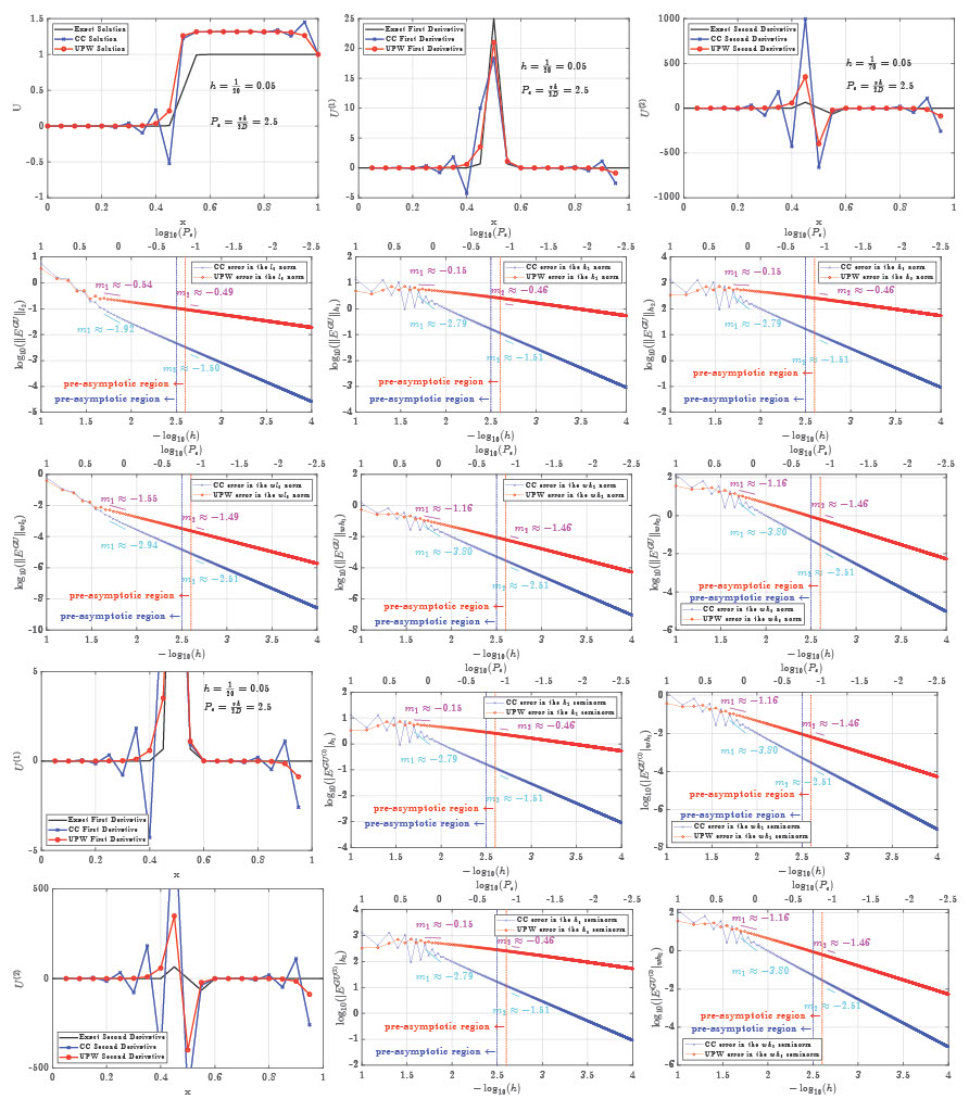
Exact and numerical solutions, their derivatives and errors in different norms and seminorms for $D=0.01$, $v=1$. Top row shows the exact and numerical solutions (left), first derivative of them (center), second derivative of them (right). Second row shows the global error in the $l_2$ (left), $h_1$ (center), $h_2$ (right) norms. Third row shows the global error in the $w{l}_2$ (left), $w{h}_1$ (center), $w{h}_2$ (right) weighted norms. Fourth row shows a zoom on the Y-axis for the first derivative (left), the global error in the $h_1$ seminorm (center) and $w{h}_1$ weighted seminorm (right). Fifth row shows a zoom on the Y-axis for the second derivative (left), the global error in the $h_2$ seminorm (center) and $w{h}_2$ weighted seminorm (right).

Figure 1 contains several subfigures grouped into five rows, where each row contains three subfigures. In the top row are shown: the exact solution together with the numerical solutions of the CC and UPW schemes (left), the first derivative of the exact and numerical solutions calculated using equation (11) for the CC scheme and equation (12) for the UPW scheme (center), and the second derivative of the exact and numerical solutions using equation (10) for both schemes (right). The derivatives of the numerical solutions were not calculated at the boundary points, since at these points the equations (11), (12) and (10) that determine the matrix of the linear system cannot be used. This has no impact on the error in the $l_2$ norm because at these points the numerical solution coincides with the exact one, since the Dirichlet boundary condition is strongly required. In general, the numerical solutions and their derivatives show a behavior similar to that of the exact solution for this local Péclet number ($P_e=\frac{\left|v\right|h}{2D}=2.5$). It can be seen that the solution of the UPW scheme is further away from the exact solution than that of the CC scheme. The behavior of the two derivatives of the UPW scheme moves away from the exact derivatives at points close to the right boundary.

In the second row of Figure 1, the global error as a function of $h$ (lower axis) and $P_e$ (upper axis) is shown for both schemes. The global error measured in the $l_2$ norm (left) is calculated using equation (16). The global error in the $h_1$ norm uses equation (18) (center), and the global error in the $h_2$ norm is calculated with equation (20) (right). For the same reasons mentioned above, all errors are calculated without considering the boundary points. The main highlight here is that in the new $h_1$ and $h_2$ norms the global error of the UPW scheme is not always monotonically decreasing as is the case with the error of the CC scheme. In these two norms the asymptotic region is reached for meshes much finer than in the $l_2$ norm. This indicates that the first and second derivatives of the UPW scheme are not very well approximated when compared to the CC scheme, although the same equation (10) was used to calculate the matrix of the linear system. Furthermore, this observation cannot be noticed by analyzing only the solution curves and the error in the $l_2$ norm, showing the benefit of comparing the numerical derivative curves and measuring the global error in the new $h_1$ and $h_2$ norms. In addition, for each scheme the approximate starting point of the asymptotic convergence region in the $l_2$ norm ($h_{00}$) is shown with a dashed vertical line, which is retained in the $h_1$ and $h_2$ norms for comparison purposes. Straight lines parallel to the curve of each global error and its approximate slope value $m$ are shown. The slope $m$ determines the actual rate of convergence of each scheme at this point $h$ (mesh). The convergence rate of the CC scheme is higher than that of the UPW scheme for all norms.

The third row of Figure 1 shows the global errors in the $w{l}_2$, $w{h}_1$ and $w{h}_2$ weighted norms using equations (17), (19) and (21). In these weighted norms the error is always monotonically decreasing. It can be noted that the asymptotic region in the $w{h}_1$ and $w{h}_2$ norms starts for more refined meshes when compared to the $w{l}_2$ norm, with the $w{h}_2$ norm being the most refined of all. In other words, the error of the second derivative is greater than that of the first derivative, which in turn is greater than the error of the solution. In addition, there is a notable difference in the error behavior for the $w{h}_1$ and $w{h}_2$ norms when compared to the $h_1$ and $h_2$ norms, indicating that the weighted norms may be more appropriate for the numerical analysis of the schemes.

The fourth row shows: a zoom on the Y-axis for the first derivative (left), the error in the $h_1$ seminorm uses equation (48) (center), and the error in the weighted $w{h}_1$ seminorm uses equation (49) (right). It can be noted that the asymptotic region in the $h_1$ and $w{h}_1$ seminorms starts for more refined meshes when compared to the $w{l}_2$ norm. Again, there is a notable difference between the behavior of the error in the $w{h}_1$ seminorm and the $h_1$ seminorm, showing that the weighted seminorm may be more appropriate for numerical analysis of the schemes.

The fifth row shows: a zoom on the Y-axis for the second derivative (left), the error in the $h_2$ seminorm uses equation (50) (center), and the error in the weighted $w{h}_2$ seminorm uses equation (51) (right). It can be noted that the asymptotic region in the $h_2$ and $w{h}_2$ seminorms starts for more refined meshes when compared to the $w{l}_2$ norm. Again, the difference between the error behavior in the $w{h}_2$ seminorm and the $h_2$ seminorm is visible, confirming that the weighted seminorm may be more appropriate for the numerical analysis of the schemes. Furthermore, with the global error measured in the $h_1$ and $h_2$ seminorms, it is possible to state that the low convergence rates of the UPW scheme in the $h_1$ and $h_2$ norms are caused by the low accuracy of the derivatives for this scheme, although the subfigures with the zoom of the derivatives show an apparently acceptable behavior.

Everything found in this model problem, whose exact solution is smooth, highlights the benefits of including in the analysis of the schemes the global error measured in the new norms and seminorms proposed in this work. Another interesting fact to highlight is that the asymptotic convergence rates of both schemes are different. The global error of the CC scheme has as asymptote the straight line with slope $m_w^{aCC}=-2.5$ for all weighted norms and weighted seminorms, while the UPW scheme has as asymptote the straight line with slope $m_w^{aUPW}=-1.5$. When weighted norms are not used, the global error of the CC scheme has as asymptote the straight line with slope $m_c^{aCC}=-1.5$ for all norms and seminorms, while the UPW scheme has as asymptote the straight line with slope $m_c^{aUPW}=-0.50$. It is possible to note that the asymptotic convergence rates verify the following relationship $m_c^{aSch}=m_w^{aSch}+1$, where for each scheme $m_w^{aSch}$ denotes the asymptotic rates measured in the weighted norms or seminorms and $m_c^{aSch}$ in the classical norms or seminorms. Furthermore, comparing the asymptotic convergence rates of both schemes for the same norm or seminorm, the following relationship $m_{\#}^{aUPW}=m_{\#}^{aCC}+1$ is verified, where $\#=c$ or $\#=w$. This last relation shows that the CC scheme has one order more in the asymptotic convergence rate than the UPW scheme.

1D cases with boundary layers

Problem with external boundary layer: Consider the equation (1) in $\Omega =]0,1[$ with constant $D$ and $v>0$, $f\left(x\right)=0$, boundary conditions $u(x=0)=1$ and $u(x=1)=0$. The exact solution of this problem $u\left(x\right)=\frac{e^{-\frac{v}{D}(1-x)}-e^{-\frac{v}{D}}}{1-e^{-\frac{v}{D}}}$ has a boundary layer near the point $x=1$ when $v>>D$, whose derivatives are $\frac{du}{dx}=\frac{v{e}^{-\frac{v}{D}(1-x)}}{D[1-e^{-\frac{v}{D}}]}$ and $\frac{d^{2}u}{d{x}^2}=\frac{v^2{e}^{-\frac{v}{D}(1-x)}}{D^2[1-e^{-\frac{v}{D}}]}$. If it is assumed that $v\ne 0$, then at least $u\in C^2\left(\Omega \right)$ as can be seen in Figure 2.

Figure 2
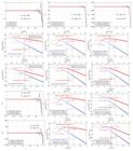
Exact and numerical solutions, their derivatives and errors in different norms and seminorms for $D=0.01$, $v=1$. Top row shows the exact and numerical solutions (left), first derivative of them (center), second derivative of them (right). Second row shows the global error in the $l_2$ (left), $h_1$ (center), $h_2$ (right) norms. Third row shows the global error in the $w{l}_2$ (left), $w{h}_1$ (center), $w{h}_2$ (right) weighted norms. Fourth row shows a zoom on the Y-axis for the first derivative (left), the global error in the $h_1$ seminorm (center) and $w{h}_1$ weighted seminorm (right). Fifth row shows a zoom on the Y-axis for the second derivative (left), the global error in the $h_2$ seminorm (center) and $w{h}_2$ weighted seminorm (right).

In the top row of Figure 2 are shown: the exact solution together with the numerical solutions of the CC and UPW schemes (left), the first derivative of the exact and numerical solutions calculated using equation (11) for the CC scheme and equation (12) for the UPW scheme (center), and the second derivative of the exact and numerical solutions using equation (10) for both schemes (right). Again, the derivatives of the numerical solutions were not calculated at the boundary points for the same reasons given in the previous model problem. The solution of the CC scheme and its derivatives show the ‘pathology’ of spurious oscillations for this local Péclet number ($P_e=2.5$), since the problem has an external boundary layer. Due to the scale of the Y-axis, it is not possible to observe these spurious oscillations for the derivatives, but they become evident with the zoom shown in the fourth and fifth rows of Figure 2. The solution of the UPW scheme and its derivatives do not present this ‘pathology’ as is already well known in the literature.

In the second row of Figure 2, the global error as a function of $h$ (lower axis) and $P_e$ (upper axis) is shown for both schemes. The global error measured in the $l_2$ norm (left) is calculated using equation (16). The global error in the $h_1$ norm uses equation (18) (center), and the global error in the $h_2$ norm is calculated with equation (20) (right). All errors are calculated without considering the boundary points. The main highlight here is that in the $l_2$ norm the error of the CC scheme is monotonically decreasing, while that of the UPW scheme is not. However, due to spurious oscillations, the error of the CC scheme is higher for meshes with $P_e>1$. For meshes with $P_e>1$, the error of the CC scheme becomes smaller than that of the UPW scheme. In the $h_1$ and $h_2$ norms, the global error of both schemes loses monoticity. The beginning of the asymptotic convergence region of the CC scheme corresponds to a coarser mesh than that of the UPW scheme, and the convergence rate of the CC scheme is higher than that of the UPW scheme for all norms. It can be noted that the asymptotic region in the $h_1$ and $h_2$ norms starts for more refined meshes ($h_{01}$ and $h_{02}$) when compared to the $l_2$ norm ($h_{00}$), i.e., $h_{02}>h_{01}>h_{00}$.

The third row of Figure 2 shows the global errors in the $w{l}_2$, $w{h}_1$ and $w{h}_2$ weighted norms using equations (17), (19) and (21). There is a notable difference in the error behavior for the $w{h}_1$ and $w{h}_2$ norms when compared to the $h_1$ and $h_2$ norms. For the UPW scheme in the $w{h}_1$ and $w{h}_2$ weighted norms there is a region where the monoticity of the error undergoes significant changes ($1⪅-{log}_{10}\left(h\right)⪅2.1$), presenting a local minimum and two local maxima. This indicates that the first and second derivatives of the UPW scheme are not well approximated in this region. The error begins to behave in a manner close to the expected asymptotic only after this region. It should be noted that a large part of this region corresponds to $P_e>1$, and this behavior is unprecedented as far as the authors know. This behavior can also be noticed by analyzing the error in the $h_1$ and $h_2$ norms. Furthermore, this behavior cannot be noticed by analyzing only the error in the $l_2$ and $w{l}_2$ norms, since it only appears in the $h_1$, $h_2$, $w{h}_1$ and $w{h}_2$ norms. On the other hand, in this same region the error of the CC scheme in the $w{h}_1$ and $w{h}_2$ weighted norms already approaches the expected asymptotic behavior. In addition to all that has been said, comparing these six norms for each scheme, it is possible to notice that the mesh parameter $h$ that produces the largest error is not the same for all norms. In other words, it is not the same mesh refinement that produces the largest error for each of these norms.

The fourth row shows: a zoom on the Y-axis for the first derivative (left), the error in the $h_1$ seminorm uses equation (48) (center), and the error in the weighted $w{h}_1$ seminorm uses equation (49) (right). With this zoom, it is possible to notice the spurious oscillations of the CC scheme. Again, there is a notable difference between the behavior of the error in the $w{h}_1$ seminorm and the $h_1$ seminorm. On the other hand, comparing the errors in the $h_1$, $w{h}_1$ norms and seminorms, it is possible to state that this unknown behavior of the global error for the UPW scheme occurs because in the region $-1⪅{log}_{10}\left(P_e\right)⪅0.5$ the first derivative of the scheme is not yet well approximated. In addition, it can be noted that the asymptotic region in the $h_1$ and $w{h}_1$ seminorms starts for more refined meshes when compared to the $w{l}_2$ norm.

The fifth row shows: a zoom on the Y-axis for the second derivative (left), the error in the $h_2$ seminorm uses equation (50) (center), and the error in the weighted $w{h}_2$ seminorm uses equation (51) (right). Again, the difference between the behavior of the global error in the $w{h}_2$ seminorm and the $h_2$ seminorm is visible. On the other hand, comparing the errors in the $h_2$, $w{h}_2$ norms and seminorms, it is possible to state that this unknown behavior of the global error for the UPW scheme occurs because in the region $-1⪅{log}_{10}\left(P_e\right)⪅0.5$ the second derivative of the scheme is not yet well approximated. In summary, in the region $0.37⪅P_e⪅1.65$ the first and second derivatives of the UPW scheme are still not well approximated, only for mesh with $P_e⪅0.37$ the derivatives begin to behave as expected for the asymptotic region. In other words, meshes with $P_e\approx 1$ do not guarantee a good approximation for the solution and the derivatives of the UPW scheme, requiring more refined meshes.

All that was found in this model problem, whose exact solution has an external boundary layer, again highlights the benefits of including in the analysis of the schemes the global error measured in the new norms and seminorms proposed in this work. Another interesting fact to highlight is that the asymptotic convergence rates of both schemes are the same as in the previous model problem, also verifying the same relationships already mentioned: $m_c^{aSch}=m_w^{aSch}+1$ and $m_{\#}^{aUPW}=m_{\#}^{aCC}+1$.

Figure 3
Exact and numerical solutions, their derivatives and errors in different norms and seminorms for $D=0.01$, $v=1$, $\bar{u}=1$ and $\beta =0.5$. Top row shows the exact and numerical solutions (left), first derivative of them (center), second derivative of them (right). Second row shows the global error in the $l_2$ (left), $h_1$ (center), $h_2$ (right) norms. Third row shows the global error in the $w{l}_2$ (left), $w{h}_1$ (center), $w{h}_2$ (right) weighted norms. Fourth row shows a zoom on the Y-axis for the first derivative (left), the global error in the $h_1$ seminorm (center) and $w{h}_1$ weighted seminorm (right). Fifth row shows a zoom on the Y-axis for the second derivative (left), the global error in the $h_2$ seminorm (center) and $w{h}_2$ weighted seminorm (right).

In the top row of Figure 3 are shown: the exact solution together with the numerical solutions of the CC and UPW schemes (left), the first derivative of the exact and numerical solutions calculated using equation (11) for the CC scheme and equation (12) for the UPW scheme (center), and the second derivative of the exact and numerical solutions using equation (10) for both schemes (right). Again, the derivatives of the numerical solutions were not calculated at the boundary points. As mentioned before, this does not impact the error in the $l_2$ norm, only the errors in the $h_1$, $h_2$, $w{h}_1$, $w{h}_2$ norms and seminorms are underestimated. The solution of the CC scheme and its derivatives show the ‘pathology’ of spurious oscillations for this Péclet number ($P_e=2.5$), since the problem has an internal boundary layer. Due to the scale of the Y-axis, it is not possible to observe these spurious oscillations for the derivatives, but they become evident with the zoom shown in the fourth and fifth rows of Figure 3. The solution of the UPW scheme and its derivatives do not present this ‘pathology’ as is already well known in the literature.

In the second row of Figure 3, the global error as a function of $h$ (lower axis) and $P_e$ (upper axis) is shown for both schemes. The global error measured in the $l_2$ norm (left) is calculated using equation (16). The global error in the $h_1$ norm uses equation (18) (center), and the global error in the $h_2$ norm is calculated with equation (20) (right). All errors are calculated without considering the boundary points. Due to spurious oscillations the error of the CC scheme is larger than the error of the UPW scheme up to a certain value of $P_e$. In the $l_2$, $h_1$ and $h_2$ norms the error of both schemes presents a similar behavior. As expected, the convergence rate of the CC scheme is greater than that of the UPW scheme in all norms for the asymptotic region.

The third row of Figure 3 shows the global errors in the $w{l}_2$, $w{h}_1$ and $w{h}_2$ weighted norms using equations (17), (19) and (21). The fourth row shows: a zoom on the Y-axis for the first derivative (left), the error in the $h_1$ seminorm uses equation (48) (center), and the error in the weighted $w{h}_1$ seminorm uses equation (49) (right). The fifth row shows: a zoom on the Y-axis for the second derivative (left), the error in the $h_2$ seminorm uses equation (50) (center), and the error in the weighted $w{h}_2$ seminorm uses equation (51) (right).

Everything found in this model problem, whose exact solution has an internal boundary layer, highlights the benefits of including in the analysis of the schemes the global error measured in the new norms and seminorms proposed in this work. Another interesting fact to highlight is that the asymptotic convergence rates of both schemes are the same as in the two previous model problems, also verifying the same relationships already mentioned: $m_c^{aSch}=m_w^{aSch}+1$ and $m_{\#}^{aUPW}=m_{\#}^{aCC}+1$.

Table I presents absolute global errors for the three model problems analyzed in 1D case. Six vector norms are used to calculate these errors. The usual norm or euclidean norm and five other new norms introduced for the first time in this study. That is, the $l_2$, $h_1$, $h_2$ norms and their respective $w{l}_2$, $w{h}_1$, $w{h}_2$ weighted norms. Errors are calculated for the two classical schemes analyzed in this study: centered and upwind. Two different values of the diffusion coefficient $D$ and three mesh parameters $h$ are used for each model problem. It is possible to note that $w{l}_2$, $w{h}_1$, $w{h}_2$ weighted norms are more appropriate than $l_2$, $h_1$, $h_2$ norms as it had already been observed in Figures 1, 2 and 3. In addition, errors in $h_1$, $h_2$ norms are larger than in $l_2$ norm, as they include the errors of the first and second derivative respectively. It should be noted that in the problem with smooth solution the errors of the second derivative for the upwind scheme are much larger than those of the centered scheme, needing very refined meshes with low Péclet number to get acceptable errors. For this type of problem the centered scheme has good accuracy for the solution, the first derivative and second derivative. In problems with boundary layers the errors of the second derivative are large for both schemes.

Table I
Global error in six norms as a benchmark for the 1D case.

$h\to P_e$	${\Vert E^{\mathrm{CC}}\Vert }_{l2}$	${\Vert E^{\mathrm{CC}}\Vert }_{h1}$	${\Vert E^{\mathrm{CC}}\Vert }_{h2}$	${\Vert E^{\mathrm{CC}}\Vert }_{wl2}$	${\Vert E^{\mathrm{CC}}\Vert }_{wh1}$	${\Vert E^{\mathrm{GU}}\Vert }_{wh2}$
	${\Vert E^{\mathrm{UPW}}\Vert }_{l2}$	${\Vert E^{\mathrm{UPW}}\Vert }_{h1}$	${\Vert E^{\mathrm{UPW}}\Vert }_{h2}$	${\Vert E^{\mathrm{UPW}}\Vert }_{wl2}$	${\Vert E^{\mathrm{UPW}}\Vert }_{wh1}$	${\Vert E^{\mathrm{UPW}}\Vert }_{wh2}$
Problem with smooth solution: D = 0.01, v = 1.
0.1 → 5.0	3.64085×10−2 5.68378×10−1	3.65066×10−2 6.31841×10−1	2.69986×10−1 2.76062×101	4.04539×10−3 6.31531×10−2	4.05629×10−3 7.02046×10−2	2.99985×10−2 3.067361728
0.02 → 1.0	3.22451×10−3 2.66262×10−1	3.26954×10−3 7.89313×10−1	5.41713×10−2 7.43089×101	6.58064×10−5 5.43392×10−3	6.67253×10−5 1.61084×10−2	1.10553×10−3 1.516509571
0.002 → 0.1	1.01923×10−4 8.52480×10−2	1.06281×10−4 7.94077×10−1	3.01391×10−3 7.89528×101	2.04256×10−7 1.70837×10−4	2.12988×10−7 1.59133×10−3	6.03990×10−6 1.58222×10−2
Problem with smooth solution: D = 0.001, v = 1.
0.01 → 5.0	1.16094×10−3 1.91273×10−1	1.16112×10−3 3.23473×10−1	2.01289×10−2 2.60863×102	1.17267×10−5 1.93205×10−3	1.17284×10−5 3.26741×10−3	2.03322×10−4 2.634984716
0.002 → 1.0	1.03826×10−4 8.58713×10−2	1.03956×10−4 7.45467×10−1	5.19409×10−3 7.40505×102	2.08069×10−7 1.72086×10−4	2.08329×10−7 1.49392×10−3	1.04090×10−5 1.483978727
0.0002 → 0.1	3.28327×10−6 2.71845×10−2	3.29673×10−6 7.89824×10−1	2.97586×10−4 7.89356×102	6.56786×10−10 5.43798×10−6	6.59478×10−10 1.57996×10−4	5.95291×10−8 1.57902×10−1
Problem with external boundary layer: D = 0.01, v = 1.
0.1 → 5.0	9.19527×10−1 9.12418×10−2	3.897894044 8.30389×10−1	3.78808×102 8.25403×101	1.02169×10−1 1.01379×10−2	4.33099×10−1 9.22655×10−2	4.20898×101 9.171148054
0.02 → 1.0	1.36591×10−1 2.21746×10−1	1.16153×101 3.249384266	1.16151×103 3.24197×102	2.78759×10−3 4.52543×10−3	2.37047×10−1 6.63139×10−2	2.37042×101 6.616269419
0.002 → 0.1	3.73969×10−3 1.05867×10−1	1.172428913 1.80439×101	1.17248×102 1.80445×103	7.49438×10−6 2.12158×10−4	2.34955×10−3 3.61603×10−2	2.34966×10−1 3.616149726
Problem with external boundary layer: D = 0.001, v = 1.
0.01 → 5.0	8.94461×10−1 9.12418×10−2	3.72447×101 8.254119849	3.72339×104 8.25361×103	9.03495×10−3 9.21635×10−4	3.76209×10−1 8.33749×10−2	3.761009×102 8.33698×101
0.002 → 1.0	1.36591×10−1 2.21746×10−1	1.16145×102 3.24188×101	1.16145×105 3.24181×104	2.73731×10−4 4.44381×10−4	2.32756×10−1 6.49676×10−2	2.32756×102 6.49661×101
0.0002 → 0.1	3.73969×10−3 1.05867×10−1	1.17242×101 1.80436×102	1.17242×104 1.80436×105	7.48089×10−7 2.11776×10−5	2.34531×10−3 3.60945×10−2	2.345316133 3.60946×101
Problem with internal boundary layer: D = 0.01, v = 1.
0.1 → 5.0	5.588840510 3.554068790	1.43144×101 4.861175790	1.31791×103 3.31692×102	6.20982×10−1 3.94896×10−1	1.590499860 5.40131×10−1	1.46435×102 3.68547×101
0.02 → 1.0	9.66171×10−2 2.52825×10−1	4.661116234 5.330358943	4.66034×102 5.32462×102	1.97177×10−3 5.15969×10−3	9.51248×10−2 1.08782×10−1	9.510914021 1.08665×101
0.002 → 0.1	2.34414×10−3 8.38739×10−2	8.26431×10−2 2.309430925	8.261404872 2.30802×102	4.69768×10−6 1.68083×10−4	1.65617×10−4 4.62811×10−3	1.65559×10−2 4.62529×10−1
Problem with internal boundary layer: D = 0.1, v = 5.
0.2 → 5.0	1.339005717 1.161718403	1.819341166 1.281276560	6.16114×101 2.70525×101	3.34751×10−1 2.90429×10−1	4.54835×10−1 3.20319×10−1	1.54028×101 6.763142791
0.04 → 1.0	9.09779×10−2 2.35363×10−1	7.72443×10−1 3.050616716	3.83611×101 1.52106×102	3.79074×10−3 9.80682×10−3	3.21851×10−2 1.27109×10−1	1.598381182 6.337782408
0.004 → 0.1	2.34414×10−3 8.38738×10−2	4.13714×10−2 1.156997805	2.065662213 5.77092×101	9.41423×10−6 3.36842×10−4	1.66150×10−4 4.64657×10−3	8.29583×10−3 2.31764×10−1

2D cases without boundary layers

Problem with smooth solution: Consider the equation (1) in $\Omega =(0,1)\times (0,1)$ with constant $D$ and $v=(v_1,v_2)$,

$$f(x,y)=\frac{D{\pi }^2}{2}[sin\left(\pi x\right)+sin\left(\pi y\right)]+\frac{\pi }{2}[v_{1}cos\left(\pi x\right)+v_{2}cos\left(\pi y\right)],$$(55)

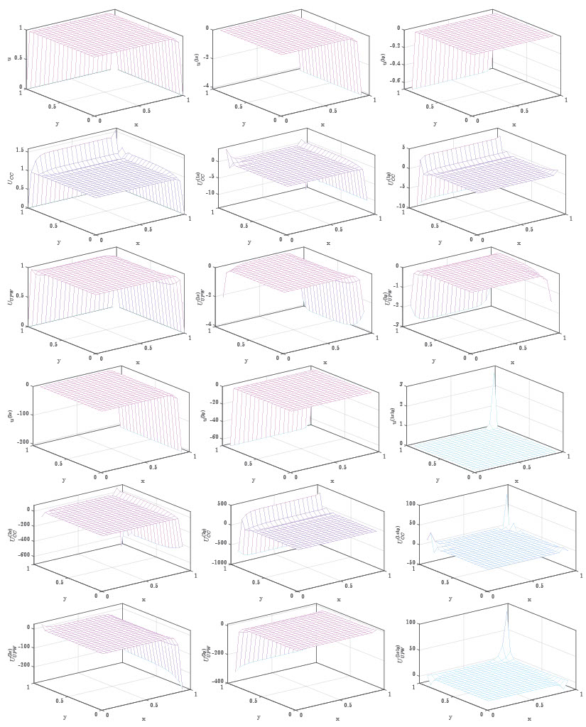
and boundary conditions such that the exact solution is $u(x,y)=\frac{1}{2}[sin\left(\pi x\right)+sin\left(\pi y\right)]\in C^{\infty }\left(\Omega \right)$. This problem is very interesting because $\frac{{\partial }^{2}u}{\partial y\partial x}=0$.

Figure 4 contains several subfigures grouped into six rows, where each row contains three subfigures. In the top row are shown: the exact solution (left), its first derivative in $x$ (center), and its first derivative in $y$ (right). The derivatives of the exact solution were not calculated at the boundary points to facilitate comparison with the derivatives of the numerical solutions. In the second row of Figure 4 are shown: the numerical solution of the CC scheme (left), its first derivative at $x$ (center), and its first derivative at $y$ (right). For the same reasons as in the 1D case, all derivatives of the numerical solutions were not calculated at the boundary points. Third row shows: the numerical solution of the UPW scheme (left), its first derivative at $x$ (center), and its first derivative at $y$ (right). Fourth row shows: the second derivative at $x$ of the exact solution (left), its second derivative at $y$ (center), and its second derivative crossed at $x$ and $y$ (right). The fifth row shows: the second derivative at $x$ of the numerical solution of the CC scheme (left), its second derivative at $y$ (center), and its second derivative crossed at $x$ and $y$ (right). Finally, the sixth row shows: the second derivative at $x$ of the numerical solution of the UPW scheme (left), its second derivative at $y$ (center), and its second derivative crossed at $x$ and $y$ (right). It can clearly be seen that the biggest difference with the exact solution for both schemes is in all second-order derivatives, but this type of comparison is more qualitative than quantitative. The first derivatives of the UPW scheme differ more from the exact ones than the first derivatives of the CC scheme, showing a greater smearing effect. Even so, the first derivatives of both schemes appear to have an acceptable accuracy. This is the type of solution comparison often presented in articles evaluating the performance of numerical methods, but with the difference that here all the derivatives of the exact and numerical solution up to the second order are presented.

Figure 4
Exact and numerical solutions, their derivatives for $D=0.02$, $v=(1,2)$, $h=0.05$ and $P_e\approx 2.8$.

Although Figure 4 presents very interesting results, Figure 5 contributes even more to the numerical analysis of both schemes, since it presents the errors measured in the $l_2$ (left of the first row), $h_1$ (center of the first row), $h_2$ (right of the first row), $w{l}_2$ (left of the second row), $w{h}_1$ (center of the second row) and $w{h}_2$ (right of the second row) norms. The derivatives of the numerical solutions were calculated using equations (29)-(30), (31)-(32) and (33)-(34), which do not include the boundary points. The main highlight here is that the global errors in the $l_2$, $h_1$ and $h_2$ norms are not monotonically decreasing for the UPW scheme in the asymptotic region of convergence. This may lead one to believe that the UPW scheme is not convergent, since the errors of the CC scheme are monotonically decreasing. However, the errors in the $w{l}_2$, $w{h}_1$ and $w{h}_2$ weighted norms are monotonically decreasing, showing that both schemes are convergent. Again, this is an argument in favor of including the errors measured in the weighted norms in the analysis. The blue and red dashed vertical lines mark the approximate starting point ($h_{00}$) of the asymptotic convergence region in the $l_2$ norm for the CC and UPW schemes respectively. These same lines were retained across all norms for comparison. The asymptotic convergence region of both schemes in the $l_2$ and $w{l}_2$ norms is reached. However, this does not occur for the $h_1$, $w{h}_1$, $h_2$ and $w{h}_2$ norms, indicating the need for finer meshes for an adequate approximation of the derivatives. This behavior is again confirmed in all seminorms of Figure 6. In addition, the convergence rates calculated with the $w{l}_2$, $w{h}_1$ and $w{h}_2$ weighted norms are closer to the theoretically expected ones a priori than those calculated with the $l_2$, $h_1$ and $h_2$ norms.

Global errors in the $l_2$, $h_1$, $h_2$, $w{l}_2$, $w{h}_1$ and $w{h}_2$ norms for $D=0.02$, $v=(1,2)$.

Figure 6
Global errors in the $h_1$, $h_2$, $w{h}_1$, $w{h}_2$ seminorms and the cross derivative for $D=0.02$, $v=(1,2)$.

Figure 6 presents the errors measured in the $h_1$ seminorm uses equation (48) (left of the first row), $h_2$ seminorm uses equation (50) (center of the first row), $w{h}_1$ seminorm uses equation (49) (left of the second row) and $w{h}_2$ seminorm uses equation (51) (center of the second row). In addition, the errors of the second cross derivative measured in the $h_2$ seminorm (right of the first row) and $w{h}_2$ seminorm (right of the second row) are presented. These last two subfigures allow us to evaluate the impact of the cross derivative on the global error of each scheme, which is another novelty of this work. As can be seen, the error increases as the approximations of the derivatives are included in the analysis. Comparing the error in the $h_1$ or $w{h}_1$ norm with the error in the $h_1$ or $w{h}_1$ seminorm, it can be concluded that the contribution of the derivatives to the global error is greater than that of the solution (error in the $l_2$ or $w{l}_2$ norm). This same conclusion remains valid when comparing the error in the $h_2$ or $w{h}_2$ norm with the error in the $h_2$ or $w{h}_2$ seminorm. Furthermore, the contribution of the cross derivative to the error in the $h_2$ or $w{h}_2$ norm and $h_2$ or $w{h}_2$ seminorm is very significant, even though this derivative is not part of the partial differential equation (PDE).

Another interesting fact to highlight is that the asymptotic convergence rates of both schemes are different. The global error of the CC scheme has as asymptote the straight line with slope $m_w^{aCC}=-3$ for all weighted norms and weighted seminorms, while the UPW scheme has as asymptote the straight line with slope $m_w^{aUPW}=-2$. When weighted norms are not used, the global error of the CC scheme has as asymptote the straight line with slope $m_c^{aCC}=-1$ for all norms and seminorms, while the UPW scheme has as asymptote the straight line with slope $m_c^{aUPW}=0$. It is possible to note that the asymptotic convergence rates verify the following relationship $m_c^{aSch}=m_w^{aSch}+2$, where for each scheme $m_w^{aSch}$ denotes the asymptotic rates measured in the weighted norms or seminorms and $m_c^{aSch}$ in the classical norms or seminorms. Furthermore, comparing the asymptotic convergence rates of both schemes for the same norm or seminorm, the following relationship $m_{\#}^{aUPW}=m_{\#}^{aCC}+1$ is verified, where $\#=c$ or $\#=w$. This last relation shows that the CC scheme has one order more in the asymptotic convergence rate than the UPW scheme.

2D cases with boundary layers

Problem with external boundary layer and advection skew to the mesh: Consider the equation (1) in $\Omega =(0,1)\times (0,1)$ with constant $D$ and $v=(v_1,v_2)$, $f(x,y)=0$, and boundary conditions such that the exact solution is $u(x,y)=1-e^{\frac{v_1}{D}(x-1)}-e^{\frac{v_2}{D}(y-1)}+e^{[\frac{v_1}{D}(x-1)+\frac{v_2}{D}(y-1)]}$, which is at least $u\in C^2\left(\Omega \right)$ as can be seen in Figure 7. This model problem presents two external boundary layers when $v_1>>D$ and $v_2>>D$, which are transversal and located near the boundaries $x=1$ and $y=1$.

Similar to the previous model problem, Figure 7 contains several results grouped into six rows, and each row contains three subfigures. In the top row are shown: the exact solution (left), its first derivative in $x$ (center), and its first derivative in $y$ (right). The derivatives of the exact solution were not calculated at the boundary points to facilitate comparison with the derivatives of the numerical solutions. In the second row of Figure 7 are shown: the numerical solution of the CC scheme (left), its first derivative at $x$ (center), and its first derivative at $y$ (right). For the same reasons as in the 1D case, all derivatives of the numerical solutions were not calculated at the boundary points. Third row shows: the numerical solution of the UPW scheme (left), its first derivative at $x$ (center), and its first derivative at $y$ (right). Fourth row shows: the second derivative at $x$ of the exact solution (left), its second derivative at $y$ (center), and its second derivative crossed at $x$ and $y$ (right). The fifth row shows: the second derivative at $x$ of the numerical solution of the CC scheme (left), its second derivative at $y$ (center), and its second derivative crossed at $x$ and $y$ (right). Finally, the sixth row shows: the second derivative at $x$ of the numerical solution of the UPW scheme (left), its second derivative at $y$ (center), and its second derivative crossed at $x$ and $y$ (right). It can clearly be seen the spurious oscillations in the solution of the CC scheme and the smearing effect in the solution of the UPW scheme. These two ‘pathologies’ also appear in all first and second order derivatives, but this type of comparison is more qualitative than quantitative.

Figure 7
Exact and numerical solutions, their derivatives for $D=0.02$, $v=(1,2)$, $h=0.05$ and $P_e\approx 2.8$.

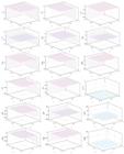
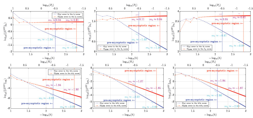
Figure 8 contributes even more to the numerical analysis of both schemes, since it presents the errors measured in the $l_2$ (left of the first row), $h_1$ (center of the first row), $h_2$ (right of the first row), $w{l}_2$ (left of the second row), $w{h}_1$ (center of the second row) and $w{h}_2$ (right of the second row) norms. The derivatives of the numerical solutions were calculated using equations (29)-(30), (31)-(32) and (33)-(34), which do not include the boundary points. The main highlight here is that the global errors in the $l_2$, $h_1$ and $h_2$ norms are not monotonically decreasing for the UPW scheme in the asymptotic region of convergence. This may lead one to believe that the UPW scheme is not convergent, since the errors of the CC scheme are monotonically decreasing in the asymptotic region of convergence. However, the errors in the $w{l}_2$, $w{h}_1$ and $w{h}_2$ weighted norms are monotonically decreasing, showing that both schemes are convergent. Again, this is an argument in favor of including the errors measured in the weighted norms in the analysis. On the other hand, the global errors in the $h_1$ and $h_2$ norms are not monotonically decreasing for the CC scheme in the pre-asymptotic region of convergence, indicating the need for finer meshes for an adequate approximation of the derivatives. In addition, the convergence rates calculated with the $w{l}_2$, $w{h}_1$ and $w{h}_2$ weighted norms are closer to the theoretically expected ones a priori than those calculated with the $l_2$, $h_1$ and $h_2$ norms. Another important highlight is that the asymptotic region of the CC scheme in the $l_2$ norm is reached for meshes with ${log}_{10}{P}_e⪅-0.5$ ($P_e⪅0.32$), while for the UPW scheme ${log}_{10}{P}_e⪅-1.3$ ($P_e⪅0.05$) is required. In other words, very refined meshes are necessary to ensure that the global error in the $l_2$ norm is in the asymptotic region of convergence. If the derivatives are considered ($h_1$ and $h_2$ norms), then even more refined meshes are necessary to ensure that the derivatives present an accuracy corresponding to the asymptotic region of convergence.

Figure 8
Global errors in the $l_2$, $h_1$, $h_2$, $w{l}_2$, $w{h}_1$ and $w{h}_2$ norms for $D=0.02$, $v=(1,2)$.

Figure 9 presents the errors measured in the $h_1$ seminorm uses equation (48) (left of the first row), $h_2$ seminorm uses equation (50) (center of the first row), $w{h}_1$ seminorm uses equation (49) (left of the second row) and $w{h}_2$ seminorm uses equation (51) (center of the second row). In addition, the errors of the second cross derivative measured in the $h_2$ seminorm (right of the first row) and $w{h}_2$ seminorm (right of the second row) are presented. These last two subfigures allow us to evaluate the impact of the cross derivative on the global error of each scheme. As can be seen, the error increases as the approximations of the derivatives are included in the analysis. Comparing the error in the $h_1$ or $w{h}_1$ norm with the error in the $h_1$ or $w{h}_1$ seminorm, it can be concluded that the contribution of the derivatives to the global error is greater than that of the solution (error in the $l_2$ or $w{l}_2$ norm). This same conclusion remains valid when comparing the error in the $h_2$ or $w{h}_2$ norm with the error in the $h_2$ or $w{h}_2$ seminorm. Furthermore, the contribution of the cross derivative to the error in the $h_2$ or $w{h}_2$ norm and $h_2$ or $w{h}_2$ seminorm is very significant, even though this derivative is not part of the PDE. Another interesting point is that the error behavior for the second cross derivative of both schemes is similar up to a certain refinement of the mesh, and subsequently for more refined meshes the error of both schemes gets closer and closer to its asymptote.

Figure 9
Global errors in the $h_1$, $h_2$, $w{h}_1$,$w{h}_2$ seminorms and the cross derivative for $D=0.02$, $v=(1,2)$.

The asymptotic convergence rates of both schemes are different and follow the same pattern as the previous model problem. The global error of the CC scheme has as asymptote the straight line with slope $m_w^{aCC}=-3$ for all weighted norms and weighted seminorms, while the UPW scheme has as asymptote the straight line with slope $m_w^{aUPW}=-2$. When weighted norms are not used, the global error of the CC scheme has as asymptote the straight line with slope $m_c^{aCC}=-1$ for all norms and seminorms, while the UPW scheme has as asymptote the straight line with slope $m_c^{aUPW}=0$. It is possible to note that the asymptotic convergence rates verify the following relationship $m_c^{aSch}=m_w^{aSch}+2$. Again, comparing the asymptotic convergence rates of both schemes for the same norm or seminorm, the following relationship $m_{\#}^{aUPW}=m_{\#}^{aCC}+1$ is verified, which indicates that the CC scheme has one order more in the asymptotic convergence rate than the UPW scheme.

Consider the equation (1) in $\Omega =(0,1)\times (0,1)$ with constant $D$ and $v=(v_1,v_2)$,

$$f=2D[{\left(\frac{v_1}{D}\right)}^2+{\left(\frac{v_2}{D}\right)}^2]{\left[u(x,y)\right]}^2[1-u(x,y)e^{-\frac{1}{D}[v_1(x-\beta )+v_2(y-\beta )]}]e^{-\frac{1}{D}[v_1(x-\beta )+v_2(y-\beta )]},$$(56)

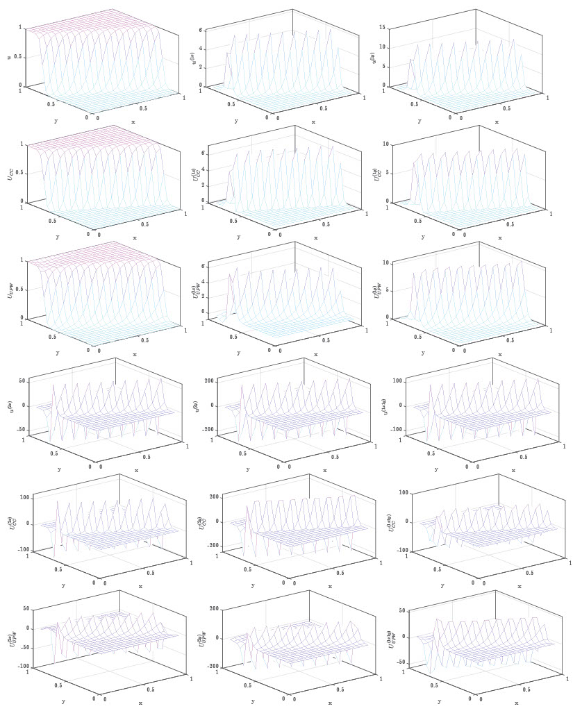
and boundary conditions such that the exact solution is $u(x,y)={[1+e^{-\frac{1}{D}[v_1(x-\beta )+v_2(y-\beta )]}]}^{-1}$, which is at least $u\in C^2\left(\Omega \right)$ as can be seen in Figure 10. This model problem presents an internal boundary layer when convection is dominant.

Figure 10 contains several results grouped into six rows, and each row contains three subfigures. In the top row are shown: the exact solution (left), its first derivative in $x$ (center), and its first derivative in $y$ (right). The derivatives of the exact solution were not calculated at the boundary points to facilitate comparison with the derivatives of the numerical solutions. In the second row of Figure 10 are shown: the numerical solution of the CC scheme (left), its first derivative at $x$ (center), and its first derivative at $y$ (right). For the same reasons as in the 1D case, all derivatives of the numerical solutions were not calculated at the boundary points. Third row shows: the numerical solution of the UPW scheme (left), its first derivative at $x$ (center), and its first derivative at $y$ (right). Fourth row shows: the second derivative at $x$ of the exact solution (left), its second derivative at $y$ (center), and its second derivative crossed at $x$ and $y$ (right). The fifth row shows: the second derivative at $x$ of the numerical solution of the CC scheme (left), its second derivative at $y$ (center), and its second derivative crossed at $x$ and $y$ (right). Finally, the sixth row shows: the second derivative at $x$ of the numerical solution of the UPW scheme (left), its second derivative at $y$ (center), and its second derivative crossed at $x$ and $y$ (right). It can clearly be seen the spurious oscillations in the solution of the CC scheme and the smearing effect in the solution of the UPW scheme. These two ‘pathologies’ also appear in all first and second order derivatives, but this type of comparison is more qualitative than quantitative.

Figure 10
Exact and numerical solutions, their derivatives for $D=0.02$, $v=(1,2)$, $\beta =0.5$, $h=0.05$ and $P_e\approx 2.8$.

Figure 11 presents the errors measured in the $l_2$ (left of the first row), $h_1$ (center of the first row), $h_2$ (right of the first row), $w{l}_2$ (left of the second row), $w{h}_1$ (center of the second row) and $w{h}_2$ (right of the second row) norms. The derivatives of the numerical solutions were calculated using equations (29)-(30), (31)-(32) and (33)-(34), which do not include the boundary points. The main highlight here is that the global errors in the $l_2$, $h_1$ and $h_2$ norms are not monotonically decreasing for the UPW scheme in the asymptotic region of convergence. This may lead one to believe that the UPW scheme is not convergent, since the errors of the CC scheme are monotonically decreasing in the asymptotic region of convergence. However, the errors in the $w{l}_2$, $w{h}_1$ and $w{h}_2$ weighted norms are monotonically decreasing, showing that both schemes are convergent. Again, this is an argument in favor of including the errors measured in the weighted norms in the analysis. In addition, the convergence rates calculated with the $w{l}_2$, $w{h}_1$ and $w{h}_2$ weighted norms are closer to the theoretically expected ones a priori than those calculated with the $l_2$, $h_1$ and $h_2$ norms.

Figure 11
Global errors in the $l_2$, $h_1$, $h_2$, $w{l}_2$, $w{h}_1$ and $w{h}_2$ norms for $D=0.02$, $v=(1,2)$.

Figure 12 presents the errors measured in the $h_1$ seminorm uses equation (48) (left of the first row), $h_2$ seminorm uses equation (50) (center of the first row), $w{h}_1$ seminorm uses equation (49) (left of the second row) and $w{h}_2$ seminorm uses equation (51) (center of the second row). In addition, the errors of the second cross derivative measured in the $h_2$ seminorm (right of the first row) and $w{h}_2$ seminorm (right of the second row) are presented. These last two subfigures allow us to evaluate the impact of the cross derivative on the global error of each scheme. As can be seen, the error increases as the approximations of the derivatives are included in the analysis. Comparing the error in the $h_1$ or $w{h}_1$ norm with the error in the $h_1$ or $w{h}_1$ seminorm, it can be concluded that the contribution of the derivatives to the global error is greater than that of the solution (error in the $l_2$ or $w{l}_2$ norm). This same conclusion remains valid when comparing the error in the $h_2$ or $w{h}_2$ norm with the error in the $h_2$ or $w{h}_2$ seminorm. Furthermore, the contribution of the cross derivative to the error in the $h_2$ or $w{h}_2$ norm and $h_2$ or $w{h}_2$ seminorm is very significant, even though this derivative is not part of the PDE.

The asymptotic convergence rates of both schemes are different and follow the same pattern as the previous model problems. The global error of the CC scheme has as asymptote the straight line with slope $m_w^{aCC}=-3$ for all weighted norms and weighted seminorms, while the UPW scheme has as asymptote the straight line with slope $m_w^{aUPW}=-2$. When weighted norms are not used, the global error of the CC scheme has as asymptote the straight line with slope $m_c^{aCC}=-1$ for all norms and seminorms, while the UPW scheme has as asymptote the straight line with slope $m_c^{aUPW}=0$. Again, it is possible to note that the asymptotic convergence rates verify the following relationship $m_c^{aSch}=m_w^{aSch}+2$. Comparing the asymptotic convergence rates of both schemes for the same norm or seminorm also verifies the same relation previously mentioned: $m_{\#}^{aUPW}=m_{\#}^{aCC}+1$, which shows that the CC scheme has one order more in the asymptotic convergence rate than the UPW scheme.

Figure 12
Global errors in the $h_1$, $h_2$, $w{h}_1$, $w{h}_2$ seminorms and the cross derivative for $D=0.02$, $v=(1,2)$.

Table II presents absolute global errors for the three model problems analyzed in 2D case. Six vector norms are used to calculate these errors. The usual norm or euclidean norm and five other new norms. That is, the $l_2$, $h_1$, $h_2$ norms and their respective $w{l}_2$, $w{h}_1$, $w{h}_2$ weighted norms. Errors are calculated for the two classical schemes analyzed in this study: centered and upwind. Two different values of the diffusion coefficient $D$ and three mesh parameters $h$ are used for each model problem. It is possible to note that $w{l}_2$, $w{h}_1$, $w{h}_2$ weighted norms are more appropriate than $l_2$, $h_1$, $h_2$ norms as it had already been observed in Figures 4, 7 and 10. In addition, errors in $h_1$, $h_2$ norms are larger than in $l_2$ norm, as they include the errors of the first and second derivative respectively. It should be noted that in the problem with smooth solution the errors of the second derivative for the upwind scheme are much larger than those of the centered scheme. In problems with boundary layers the errors of the second derivative are large for both schemes.

Table II
Global error in six norms as a benchmark for the 2D case.

h, $p_e$	$\Vert E^{\text{CC}}\Vert l_2$, $\Vert E^{\text{UPW}}\Vert l_2$	$\Vert E^{\text{CC}}\Vert h_1$, $\Vert E^{\text{UPW}}\Vert h_1$	$\Vert E^{\text{CC}}\Vert h_2$, $\Vert E^{\text{UPW}}\Vert h_2$	$\Vert E^{\text{CC}}\Vert {\mathrm{w\; l}}_2$, $\Vert E^{\text{UPW}}\Vert {\mathrm{w\; l}}_2$	$\Vert E^{\text{CC}}\Vert {\mathrm{w\; h}}_1$, $\Vert E^{\text{UPW}}\Vert {\mathrm{w\; h}}_1$	$\Vert E^{\text{GU}}\Vert {\mathrm{w\; h}}_2$,$\Vert E^{\text{UPW}}\Vert {\mathrm{w\; h}}_2$
	Problem with smooth solution: $D=0.02,v=(1,2)$
0.018181818 / 1.016394535	1.07455×10⁻² / 1.18959	4.03918×10⁻² / 5.28765	2.21253 / 3.79997×10²	3.42653×10⁻⁶ / 3.79333×10⁻⁴	1.28800×10⁻⁵ / 1.68611×10⁻³	7.05526×10⁻⁴ / 1.21172×10⁻¹
0.0018018018 / 0.100723782	1.06476×10⁻³ / 1.22746	5.27423×10⁻³ / 1.30370×10¹	3.77710×10⁻¹ / 1.16313×10³	3.44432×10⁻⁹ / 3.97061×10⁻⁶	1.70612×10⁻⁸ / 4.21724×10⁻⁵	1.22182×10⁻⁶ / 3.76252×10⁻³
Problem with smooth solution: $D=0.002,v=(1,2)$
0.001 / 0.559016994	6.42071×10⁻⁴ / 1.29028	7.53284×10⁻³ / 2.26437×10¹	6.26101 / 1.96258×10⁴	6.40789×10⁻¹⁰ / 1.28769×10⁻⁶	7.51779×10⁻⁹ / 2.25985×10⁻⁵	6.24851×10⁻⁶ / 1.95866×10⁻²
Problem with external boundary layer: $D=0.02,v=(1,2)$
0.0018018018 / 0.100723782	7.79735×10⁻² / 2.8550	2.39500×10¹ / 4.42838×10²	2.36740×10³ / 4.17801×10⁴	2.52230×10⁻⁷ / 9.23551×10⁻⁶	7.74741×10⁻⁵ / 1.43250×10⁻³	7.65814×10⁻³ / 1.35151×10⁻¹
Problem with internal boundary layer: $D=0.2,v=(5,10)$
0.003571428 / 0.099824463	2.76336×10⁻² / 1.14993	8.25561×10⁻¹ / 2.15842×10¹	5.67455×10¹ / 1.09510×10³	3.49965×10⁻⁷ / 1.45633×10⁻⁵	1.04553×10⁻⁵ / 2.73353×10⁻⁴	7.18652×10⁻⁴ / 1.38688×10⁻²

For qualitative comparison purposes, the solutions of the two cases for the model problem with internal boundary layer are presented. Figure 10 shows the solutions and their derivatives for the first case ($D=0.02$, $v=(1,2)$), while Figure 13 presents the solutions and their derivatives for the second case ($D=0.2$, $v=(5,10)$). In both figures, a grid of $21\times 21$ nodes is used.

Figure 13
Exact and numerical solutions, their derivatives for $D=0.2$, $v=(5,10)$, $\beta =0.5$, $h=0.05$ and $P_e\approx 1.39$.

To conclude the results and discussion section, it should be emphasized that only the global errors measured in the weighted norms and seminorms always have a monotonic decreasing convergence in the asymptotic region. That is, the global error tends to zero when $h$ tends to zero for all $h>h_{0m}$, where $h_{0m}$ denotes the starting point of the asymptotic convergence region for each norm $m$. Meshes with $h>h_{0m}$ belong to the pre-asymptotic region, where there is no guarantee of monotonic convergence always. In cases where the exact solution is smooth, the global error may present monoticity in the pre-asymptotic region for the $l_2$ or $w{l}_2$ norm (Figures 1, 5, 6). However, this monoticity in the pre-asymptotic region is lost in cases of exact solutions with a boundary layer. It is in this pre-asymptotic region where the spurious oscillations of the schemes appear, that is, in this region the stability of the scheme is very different from that which occurs in the asymptotic region. For all cases presented in this analysis (1D and 2D), the starting point of the asymptotic region in the $l_2$ norm ($h_{00}$) always corresponds to a coarser mesh than the starting point of the asymptotic region in the $h_1$ norm ($h_{01}$), which in turn always corresponds to a coarser mesh than the starting point of the asymptotic region in the $h_2$ norm ($h_{02}$). This statement is also valid for weighted norms and for all seminorms ($h_{02}\le h_{01}\le h_{00}$). Therefore, a mesh that guarantees an acceptable approximation for the solution $u$ does not guarantee an acceptable approximation for the derivatives of $u$.

The global error can be estimated a priori or calculated a posteriori. In general, a priori estimates of the global error do not provide a good characterization of the scheme’s performance in the pre-asymptotic region. This is because in a priori estimates it is common to assume that the derivatives of the exact solution are fairly ‘regular’ and bounded functions. Thus, a priori estimates determine for each scheme an asymptotic bound of the global error for the asymptotic region described by equation ((57)).

$${\parallel E^{G{U}_{Sch}}\parallel }_{\#}\le C{\parallel u\parallel }_{\#}{h}^{m_{\#}^{aSch}},$$(57)

where $C>0$ is a constant, $h$ is the grid parameter, $\#$ denotes the chosen norm, and $m_{\#}^{aSch}$ denotes the asymptotic convergence rate in that norm. Therefore, the actual global error will be close to this asymptote only in cases where the problem data (domain region $\Omega \cup \partial \Omega$, source $f$, boundary conditions, PDE coefficients $D$ and $v$) guarantee that the derivatives of the exact solution verify the assumptions of ‘regularity’ and boundedness assumed a priori. The smooth exact solutions presented here are examples where the global error presents a behavior similar to that of the a priori estimates in both pre-asymptotic and asymptotic regions if the $w{l}_2$ weighted norm is used. However, the exact solutions with boundary layers presented here are examples where the global error behaves close to the a priori estimate only after a certain refinement of the mesh (asymptotic region).

On the other hand, the a posteriori calculation of the global error allows a detailed characterization of both the pre-asymptotic and asymptotic regions. However, in order to perform a good a posteriori analysis, it is important to know both the exact and the numerical solution. The exact solutions presented here allowed us to calculate the actual global error (exact if round-off is disregarded) a posteriori, and thus determine the actual convergence rate of each scheme. It should be emphasized that even in the asymptotic region of convergence, this convergence rate is not constant, since it presents a smooth monotonic variation that has as its asymptote the convergence rate obtained by the a priori estimate. This a posteriori study of the global error allowed us to find for each scheme the following relationship between the asymptotic convergence rates measured in the weighted norms and the classical ones

$$m_c^{aSch}=m_w^{aSch}+\mathrm{\text{dimension}}\left(\Omega \right),$$(58)

where for each scheme $m_w^{aSch}$ denotes the asymptotic rates measured in the weighted norms or seminorms, $m_c^{aSch}$ in the classical norms or seminorms, and $\mathrm{\text{dimension}}\left(\Omega \right)=1$ for the 1D case and $2$ for the 2D case.

Finally, the norms and seminorms introduced here can be applied to any finite-dimensional vector, and not only to vectors obtained by solving the PDE with finite differences. This is because a vector is an array of numbers, where each number represents the coordinate or component of the vector. The order of the components is not the most important, since it depends on the choice of the reference system, and this order can be modified with elementary transformations. Therefore, the difference between the coordinates of the vector can be defined, which can be seen as some kind of finite difference, whose interpretation will depend on what the components of the generic vector represent. When this finite difference can be infinitesimal, we obtain the traditional concept of derivative; otherwise, we can only define the finite or non-infinitesimal difference. Therefore, these new norms and seminorms applied to any generic vector allow us to estimate different variations that may occur in this vector, and these are new properties of the vector that can be analyzed. These new properties are different from the property estimated or measured by the usual Euclidean norm, since the usual norm allows us to analyze the length of the vector, but not any type of variation that may exist between the components of the vector. Note that $\parallel U{\parallel }_{h_1}\le \parallel U{\parallel }_{l_2}+{\left|U^{\left(1\right)}\right|}_{h_1}$, that is, the $h_1$ norm estimates a new length for the vector $U$, which is upper bound by the sum of the Euclidean length with a length that represents a variation of the vector $U$. Similarly, $\parallel U{\parallel }_{h_2}\le \parallel U{\parallel }_{l_2}+{\left|U^{\left(1\right)}\right|}_{h_1}+{\left|U^{\left(2\right)}\right|}_{h_2}$ and so on. Thus, these new norms and seminorms will find application in many branches of mathematics, physics and engineering. The first application was presented in this paper.

CONCLUSIONS

For the first time in the finite difference framework, the new $h_1$ and $h_2$ vector norms and new $h_1$ and $h_2$ vector seminorms are introduced. These norms and seminorms are analogous to the $H^1$ and $H^2$ norms and seminorms used in the finite element framework. Although the $l_2$, $h_1$ and $h_2$ norms brought much interesting and novel information to the study of the performance of the schemes, the $w{l}_2$, $w{h}_1$ and $w{h}_2$ weighted norms added even more novelty, since with them it was possible to observe convergences of the schemes similar to what should be expected theoretically a priori. Furthermore, the new $h_1$, $h_2$, $w{h}_1$ and $w{h}_2$ seminorms allow the impact on the global error of the derivatives of each scheme to be assessed separately, and this is a completely new tool in the finite difference framework. These norms and seminorms and their weighted versions are valid for uniform and non-uniform meshes. Numerical results indicate that a mesh that guarantees an acceptable approximation for the solution $u$ does not guarantee an acceptable approximation for the derivatives of $u$. For this reason non-uniform meshes and new schemes will be analyzed in future articles, research on which is already underway.

Thus, the finite difference framework now has new tools analogous to the finite element framework to analyze the methods, of course observing the differences and peculiarities of each framework. Both methodologies have a robust mathematical foundation. The finite element method is supported by functional analysis, while the finite difference method is supported by numerical analysis. The above is not intended to establish any type of competition between the two methodologies. Quite the contrary, both methodologies are two different approaches to numerically solving PDEs, which can complement each other, since each of them has the so-called ‘advantages’ and ‘disadvantages’. For example, in Santos et al. (2022), a mixed approach was developed to take advantage of some ‘advantages’ of both methodologies. In addition, a good example to note the complementarity of both methodologies can be seen in the finite volume method, since it uses ingredients from both methodologies in its formulation: volume integrals and difference formulas to approximate the flows in each volume.

On the other hand, exact solutions with boundary layers are proposed as benchmarks together with the errors in the new vector norms of two classical finite difference schemes. The relevance of these exact solutions goes beyond the numerical analysis of each scheme. For example, these exact solutions can be used in the verification and validation of computer codes. Furthermore, they can also be used in the finite element and finite volume framework.

It is clear that this paper introduces a paradigm shift in the framework of finite differences. It should be said that the usefulness of these new norms and seminorms is not limited to the results presented here. For example, in the future it will be possible to make theoretical estimates a priori of the global error in the new norms and seminorms, further enriching the numerical analysis in the finite difference framework. Furthermore, all of the above can be extended to the finite volume framework, since this method uses finite difference formulas to approximate the flows in each volume. On the other hand, this work together with the Complete Centered Finite Difference Method, introduced by Alvarez et al. (2024), allows us to glimpse new horizons in the robust and very useful finite difference framework.

ACKNOWLEDGMENTS

This work was supported by the Universidade Federal Fluminense and the Coordenação de Aperfeiçoamento de Pessoal de Nível Superior - CAPES - Brazil, and dedicated to the Brazilian People and the memory of Leonhard Paul Euler.

REFERENCES

• ADAMS RA & FOURNIER JJF. 2003. Sobolev Spaces. Elsevier.
• ALMEIDA JO, LOBÃO DC, STAMPA CS & ALVAREZ GB. 2018. Multi-block technique applied to Navier-Stokes equations in two dimensions. Semin Ciênc Exatas Tecnol 39(2): 115-124. doi:10.5433/1679-0375.2018v39n2p115.
• ALMEIDA RG, ALVAREZ GB, HERNÁNDEZ CT & SOUSA PAP. 2021. Some mathematical comments about the Analytic Hierarchy Process: Part II - Practical analysis. Pesqui Ensino Ciênc Exatas Nat 5: e1820. doi:10.29215/pecen.v5i0.1820.
• ALVAREZ GB, ALMEIDA RG, HERNÁNDEZ CT & SOUSA PAP. 2021. Some mathematical comments about the analytic hierarchy process: Part I - theoretical analysis. J Multi-Criteria Decis Anal 28(5-6): 296-310. doi:10.1002/mcda.1762.
• ALVAREZ GB, ALMEIDA RG, HERNÁNDEZ CT & SOUSA PAP. 2025. The synthesis of the AHP as a well-posed mathematical problem and matrix norms appropriate for sensitivity analysis via condition number. Int J Math Oper Res 30(1): 111-134. doi:10.1504/IJMOR.2025.144549.
• ALVAREZ GB, BENTO NJS, NEVES TN, SANTOS FS, SILVA GC & SOUSA PAP. 2017. Numerical study of the influence of electrode arrangements in electrokinetic remediation technique. Environ Sci Pollut Res 24: 26424-26435. doi:10.1007/s11356-017-0017-z.
• ALVAREZ GB, NUNES HF & MENEZES WA. 2024. Complete centered finite difference method for Helmholtz equation. An Acad Bras Cienc 96(4): e20240522. doi:10.1590/0001-3765202420240522.
• BERMÚDEZ PR, SOUSA FV, LOBÃO DC, ALVAREZ GB & ALONSO BV. 2021. Hugoniot–Maslov Chain for Shock Waves in Buckley–Leverett Equations. Math Notes 110(5): 738-753. doi:10.1134/S0001434621110110.
• BROOKS AN & HUGHES TJR. 1982. Streamline upwind/Petrov-Galerkin formulations for convection dominated flows with particular emphasis on the incompressible Navier-Stokes equations. Comput Methods Appl Mech Engrg 32(1-3): 199-259.
• CARMO EGD & ALVAREZ GB. 2003. A new stabilized finite element formulation for scalar convection–diffusion problems: the streamline and approximate upwind/Petrov–Galerkin method. Comput Methods Appl Mech Engrg 192(31-32): 3379-3396. doi:10.1016/S0045-7825(03)00292-5.
• CARMO EGD & ALVAREZ GB. 2004. A new upwind function in stabilized finite element formulations, using linear and quadratic elements for scalar convection–diffusion problems. Comput Methods Appl Mech Engrg 193(23-26): 2383-2402. doi:10.1016/j.cma.2004.01.015.
• COURANT R, ISAACSON E & REES M. 1952. On the solution of nonlinear hyperbolic differential equations by finite differences. Commun Pur Appl Math 5(3): 243-255.
• EVANS LC. 2010. Partial Differential Equations. AMS - American Mathematical Society.
• GALEÃO AC & CARMO EGD. 1988. A consistent approximate upwind Petrov-Galerkin method for convection-dominated problems. Comput Methods Appl Mech Engrg 68(1): 83-95.
• GILAT A. 2014. MATLAB: An Introduction with Applications. Wiley.
• IVANOVA NM. 2008. Exact Solutions of Diffusion-Convection Equations. Dyn PDE 5(2): 139-171.
• JESUS JC, CHRISTO EDS, GARCIA VDS & ALVAREZ GB. 2016. Time Series Analysis For Modeling Of Glioma Growth In Response To Radiotherapy. IEEE Lat Am Trans 14(3): 1532-1537. doi:10.1109/TLA.2016.7459646.
• LEBEDEV LP, VOROVICH II & GLADWELL GML. 2002. Functional Analysis: Applications in Mechanics and Inverse Problems. Springer.
• LEVEQUE R. 2007. Finite Difference Methods for Ordinary and Partial Differential Equations: Steady-State and Time-Dependent Problems. SIAM.
• MACHADO BS, ALVAREZ GB & LOBÃO DC. 2023. Reactive-Advective-Diffusive Models for the Growth of Gliomas Treated with Radiotherapy. Semin Cienc Exatas Tecnol 44: e47321. doi:10.5433/1679-0375.2023.v44.47321.
• PORTEGIES JM & DUITS R. 2017. New exact and numerical solutions of the (convection-)diffusion kernels on SE(3). Differ Geom Appl 53: 182-219.
• RAITHBY GD. 1976. A critical evaluation of upstream differencing applied to problems involving fluid flow. Comput Methods Appl Mech Engrg 9(1): 75-103.
• ROCKNE R, ALVORD EC, ROCKHILL JK & SWANSON KR. 2009. A mathematical model for brain tumor response to radiation therapy. J Math Biol 58: 561-578.
• SANTOS MFF, DUTRA DO CARMO EG, FONTES JUNIOR EF & MANSUR WJ. 2022. A scheme for the analysis of primal stationary boundary value problems based on FE/FD multi-method. Finite Elem Anal Des 209: 103809.
• SILVA JJ. 2014. Modelagem computacional aplicada ao tratamento de câncer via medicina nuclear. Dissertação de Mestrado, Programa de Pós-graduação em Modelagem Computacional em Ciência e Tecnologia. Universidade Federal Fluminense, Volta Redonda, Rio de Janeiro, 80 p. (Unpublished).
• STYNES M & STYNES D. 2018. Convection Diffusion Problems: An Introduction to Their Analysis and Numerical Solution. AMS - American Mathematical Society.
• WOLFRAM S. 2015. An Elementary Introduction to the Wolfram Language. Champaign: Wolfram Media Inc.

Publication Dates

• Publication in this collection
  28 Nov 2025
• Date of issue
  2025

History

• Received
  03 Dec 2024
• Accepted
  20 Apr 2025