Wake modeling and simulation of a real scale wind turbine using large eddy simulation and dynamic adaptive mesh refinement

Abstract

Wind energy has gained visibility in terms of progress and potential worldwide. In this context, scientific research in wind energy has shown significant progress, particularly in the development of computational fluid dynamics approaches that resolve the real scale wind turbines. The present study aims to apply Large Eddy Simulation (LES) to provide crucial spatial and temporal information on the flowfield surrounding a full-scale NREL 5 MW wind turbine in order to investigate the following: (i) wind turbine-generated wakes and their effects, (ii) interactions between the wind and turbine in terms of power generation, and (iii) wake effects for back to back turbines related to energy production efficiency. The numerical framework used in the simulations performs LES under a block-structured mesh that is dynamically refined to increase accuracy and reduce computational costs. The simulated 5MW NREL presented lower recovery velocities around the hub-height centerline in the near wake compared to other selected numerical results, which could be attributed to the simplification of the blade resolving geometry applied in the previous studies. Despite that, most results presented differences lower than ​10%​ among the profiles. In addition, the power generation is validated with NREL experimental data with a difference of around ​3.5%​.

Key words
Large eddy simulation; immersed boundary method; adaptive mesh refinement; wind turbine wakes; wind turbine

INTRODUCTION

In recent decades, the world’s economic growth has led to an increase in energy demand. However, relying on combustion-based energy generation and the consumption of fossil fuels has become a major environmental concern. This is due to the fact that increased energy consumption not only depletes energy resources but also contributes to global warming and the greenhouse effect through emissions generated by burning fossil fuels. To address this issue, renewable energy resources such as solar, hydropower, and wind are being utilized to meet the growing energy requirement. Among these resources, wind energy has proven to be advantageous as it has undergone significant technological development and has gained a significant share of the energy market (Leung & Yang 2012, Kılkış et al. 2018, Edelenbosch et al. 2017).

When generating wind energy, the wind turbine generator (WTG) converts the kinetic energy of the wind passing through the turbine’s swept area into mechanical torque on the rotor hub. Currently, if manufacturer’s power curves are turned into the standard power coefficient, Cp, then the maximum is around 0.50. The amount of energy produced by a wind farm depends on various factors, such as turbine efficiency, wind availability, wind pattern characteristics, and turbine layout. To improve energy yield, it is crucial to carefully design large wind farm layouts, which requires a deep understanding of wind turbine aerodynamic behavior, wake effects, and the impact of specific wind-related parameters and coefficients on the turbine (Mo et al. 2013, Vermeer et al. 2003).

In an analysis conducted by Vermeer et al. (2003), some of the most popular analytical models were examined for estimating wake development, interaction, and superposition. The study highlights that simplified empirical models may not be capable to accurately represent the flow field in the wake. The commonly used wake model developed by Jensen (1983) considers wind speed deficit occurring only axially with the incoming wind, which is one-dimensional. However, wind speed deficit occurs both in the axial and radial wind directions. To address this, Frandsen et al. (2006) developed a circular wake model, which assumes an imposed wind speed deficit extending until striking the terrain or sideways wakes. This model also considers a top-hat shape for the velocity distribution in the wake cross-section. The model developed by Larsen (1988) uses Prandtl’s turbulent boundary layer equations, where the wind speed deficit incorporates both perpendicular and longitudinal distance from the wind turbine. It can estimate the velocity distribution in cross-sections at various longitudinal distances downstream from the turbine.

Arithmetic wake models, which are based on semi-analytical equations, have shown improvement over time. However, they are still not as accurate as more recent computational models that use computational fluid dynamics (CFD) to simulate the wake flow field, as discussed by Wang et al. (2016). In large wind farm projects, numerical modeling of the flow around turbines using CFD is becoming increasingly important in optimizing the energy efficiency of wind farms by properly resolving turbine wake effects. Various CFD studies have been conducted on stand-alone wind turbines, such as Mo et al. (2013) that used the commercial ANSYS FLUENT® package with the Smagorinsky-Lilly sub-grid turbulence model. The boundary between the near and far wake is suggested to be the average location between the starting and ending of the vortex wake breakdown process. Other researchers, such as Sedaghatizadeh et al. (2018), have also used ANSYS FLUENT® LES with the dynamic Smagorinsky-Lilly model to predict the wake diameter or velocity deficit in specific areas. Syed Ahmed Kabir & Ng (2019) employed unsteady Reynolds-Averaged NavierStokes (URANS) using ​k − ϵ​​ turbulence closure model with ANSYS FLUENT®, and concluded that velocity and turbulence intensity recovery is essential in modeling the wind farm layout.

In a study by Regodeseves & Morros (2021), simulations were conducted on the MEXICO wind turbine experiments to examine the effects of the nacelle and tower on the induction region, rotor, and near-wake. The simulations utilized the URANS approach with the SST ​k − ω​​ turbulence model and the sliding mesh method to rotate the blades. It was found that the tower had minimal impact on the blades due to the wind turbine’s large rotor overhang. Naderi et al. (2018) performed a study that applied the actuator disc (AD) model to incorporate operational and geometrical characteristics into the simulation, such as airfoil class, angular velocity, twist, and chord distribution. The results showed that the standard ​k − ϵ​​ model performed better than the RNG ​k − ϵ​​ turbulence model in terms of normalized output power. In a recent work by Wang et al. (2022), LES coupled with the actuator line method (ALM) was used to simulate the flow field around a micro wind turbine. The authors proposed new techniques for assessing the wind turbine’s rotor power coefficient and wake recovery length from an energy-based perspective. They concluded that this method could be used in transient velocity field conditions.

Improvements on wind turbine CFD simulation is still required, concerning the necessity of more detailed information on the development of the near wake. This is important for making wind farm layouts more efficient. Most of the previous studies that use simplified models did not properly simulate the near-wake dynamics due to inadequate spatial resolution of the wake region. To address this issue, we developed a numerical method that uses advanced CFD techniques such as adaptive mesh refinement (AMR) and the immersed boundary method (IBM) to efficiently resolve the interaction between blades and the tower as well as the evolution of the near-wake flow. This study aims to demonstrate the accuracy and computational efficiency of these techniques through a large eddy simulation of a fully-resolved NREL 5MW wind turbine. The study focuses on two main analyses: (i) the interaction between the wind and the wind turbine blade and (ii) the impact of wind turbine-generated wakes on downstream structures.

The article is organized as follows: the methodology section presents the numerical framework, governing equations, and numerical methods used in the research, and also the computational and boundary conditions. The results and discussion section analyzes the wake velocity field downstream of the NREL 5 MW turbine. The conclusion section summarizes the main contributions of the study and their significance.

MATERIALS AND METHODS

Numerical framework

This study employs the immersed boundary (IB) method to analyze the intricate design of wind turbines (Vedovoto et al. 2015, Neto et al. 2019, Souza et al. 2022). This method requires two separate grids: a block-structured Eulerian domain where the transport equations are solved using a finite volume approach with second-order discretization, and an unstructured Lagrangian domain representing the immersed geometry. Various IB methods are detailed in several reviews on the subject (Peskin 2002, Mittal & Iaccarino 2005, Iaccarino & Verzicco 2003, Uzgoren et al. 2007, Sotiropoulos & Yang 2014, Hou et al. 2012, Mohammadi et al. 2018). The force calculation step (implicit or explicit) and the interpolation step (diffuse or sharp) are the main differences between the different IB methods presented in the literature. Combining an IB method with a block-structured Cartesian mesh and AMR enables efficient solvers to be used within Cartesian blocks while allowing for more efficient refinement of the mesh only in regions required by the flow characteristics. The numerical framework used for this study is MFSim, developed in the Fluid Mechanics Laboratory of the Federal University of Uberlândia, Brazil. The code has been developed into a multi-disciplinary code for simulating 3D problems involving turbulent flows (Damasceno et al. 2015), fluid-structure interaction (Neto et al. 2019, Souza et al. 2022, Morales et al. 2023), multiphase flows (Barbi et al. 2018, Pinheiro et al. 2019, 2021, Mota et al. 2023), gas-solid and gas-liquid flows (Santos 2019), and chemically-reactive flows (Damasceno et al. 2018, Castro et al. 2021).

Mathematical and numerical modeling

In order to study the aerodynamics of wind turbines, we utilize the Navier Stokes equations to determine the velocity and pressure fields. To solve these equations, we employ the LES method, which is effective for simulating wind turbines because it calculates larger scales of energy while modeling smaller scales using a sub-grid scale model. It’s important to note that the size of the wind turbine blade plays a significant role in the turbulent structures responsible for most of the momentum transportation in the large scale.

In Cartesian coordinates and using index notation, for ​i, j = 1,2, 3​, the mass balance model for an incompressible fluid is given by:

$$\frac{\mathrm{\partial }{u}_i}{\mathrm{\partial }{x}_i}=0$$ (1)

where ​​​ui​​​​​​(​​m/ s​​)​​​​ is the ​i​​ component of the velocity vector. The linear momentum balance equation for an incompressible and Newtonian fluid is given by:

$$\frac{\mathrm{\partial }\rho u_i}{\mathrm{\partial }t}+\frac{\mathrm{\partial }\rho u_j{u}_i}{\mathrm{\partial }{x}_j}=-\frac{\mathrm{\partial }p}{\mathrm{\partial }{x}_i}+\frac{\mathrm{\partial }}{\mathrm{\partial }{x}_j}\left[\mu (\frac{\mathrm{\partial }{u}_i}{\mathrm{\partial }{x}_j}+\frac{\mathrm{\partial }{u}_j}{\mathrm{\partial }{x}_i})\right]+f_i$$ (2)

In this equation, ​p​​(N / ​m​​​​ 2​)​​ is the pressure, ​ρ​​(kg / ​m​​​​ 3​)​​ is the density, ​μ​​ ​​​(​​kg / ms​)​​​​ is the dynamic viscosity and ​​fi​​​​​​(N / ​m​​ 3​)​​ is the ​​i​​​​ th ​​ component of the Eulerian dynamic force vector representing the immersed boundary method.

To obtain the equations for the filtered velocities, the LES filtering process is applied over the mass and momentum balance equations, assuming cumulative property over both operators and considering negligible density variations. The resulting equations can be expressed as:

$$\frac{\mathrm{\partial }{\overline{u}}_i}{\mathrm{\partial }{x}_i}=0$$ (3)

​​​$$\frac{\mathrm{\partial }{\overline{u}}_i}{\mathrm{\partial }t}+\frac{\mathrm{\partial }({\overline{u}}_i{\overline{u}}_j)}{\mathrm{\partial }{x}_j}=-\frac{1}{\rho }\frac{\mathrm{\partial }\overline{p}}{\mathrm{\partial }{x}_i}+\frac{\mathrm{\partial }}{\mathrm{\partial }{x}_j}[\nu (\frac{\mathrm{\partial }{\overline{u}}_i}{\mathrm{\partial }{x}_j}+\frac{\mathrm{\partial }{\overline{u}}_j}{\mathrm{\partial }{x}_i})-{\tau }_{ij}]+f_i$$ (4)

where ​ν​​(​m​​​​ 2​ / s)​​ is the kinematic viscosity.

Note that the filtering process introduces a new variable in the second last term of the right-hand side of the momentum equation, Eq. (4). This term is a sub-filter tensor known as Reynolds Stress Tensor (RST), which represents the contribution of the dynamics of the sub-filter turbulent fluctuations on the resolved scales of LES, written as:

$${\tau }_{ij}={\nu }_t(\frac{\mathrm{\partial }{\overline{u}}_i}{\mathrm{\partial }{x}_j}+\frac{\mathrm{\partial }{\overline{u}}_j}{\mathrm{\partial }{x}_i})$$ (5)

where ​​νt​​​​​​ is the subgrid kinematic viscosity. For the simulation of turbulent flows with a high Reynolds number, the LES method was used with the Germano dynamic subgrid-scale model (Germano et al. 1991, Lilly 1992). The turbulent viscosity is calculated using the tensor strain rate ​​Sij​​​​​​, the length scale ​Δ​, which is usually defined by the mesh size and from the proportionality function ​​c​​(​​​ → x ​, t​​)​​​​. The turbulent viscosity is calculated using Eq. (6):

$${\nu }_t=c(\overrightarrow{x},t){\mathrm{\Delta }}^2\left|\overline{S}\right|$$ (6)

where, the strain rate tensor modulus is determined by:

$$\left|\overline{S}\right|=\sqrt{2S_{ij}{S}_{ij}}$$ (7)

and,

$$S_{ij}=\frac{1}{2}(\frac{\mathrm{\partial }{\overline{u}}_i}{\mathrm{\partial }{x}_j}+\frac{\mathrm{\partial }{\overline{u}}_j}{\mathrm{\partial }{x}_i})$$ (8)

The proportionality function is calculated using Eq. (9):

​​​$$c(\overrightarrow{x},t)=-\frac{1}{2}\frac{L_{ij}{M}_{ij}}{M_{ij}{M}_{ij}}$$ ​​​ (9)

Finally, the other tensors of the model are calculated using Eq. 10 and Eq. (11):

​​​ ​​ ​​​​$$L_{ij}=T_{ij}-{\hat{\tau }}_{ij}={\overline{u}}_i{\overline{u}}_j-{\hat{\overline{u}}}_i{\hat{\overline{u}}}_j$$ (10)

$$M_{ij}={\overline{\mathrm{\Delta }}}^2|\hat{\overline{S}}|{\hat{\overline{S}}}_{ij}-{\mathrm{\Delta }}^2|\overline{S}|{\overline{S}}_{ij}$$ (11)

where ​​L_ij​​​​​​ is the Leonard tensor and ​​M_ij​​​​​​​​​ is the Germano identity (Lilly 1992). The Lagrangian formulation of the work is based on the IB method framework, which is connected to the Eulerian formulation represented by the LES method. This resulting approach is advantageous because it can simulate flows over complex geometries by using a Cartesian grid to solve the balance and transport equations in the Eulerian domain and coupling the two frames through the use of source terms. In this work, the method used is modified the multi-direct forcing method presented in Wang et al. (2008), with the modifications fully described in Vedovoto et al. (2015). The method involves an iterative process of the direct forcing method, which is explained in detail in Neto et al. (2019) and Souza et al. (2022).

The force term, ​​fi​​​​​​, in the momentum equation (Eq. 4) controls the definition of the immersed boundaries. A distribution function is used to calculate this force as:

$$f_i(\overrightarrow{x})=\sum _K\overrightarrow{F}({\overrightarrow{x}}_K)D_{ij}(\overrightarrow{x}-{\overrightarrow{x}}_K)\mathrm{\Delta }V({\overrightarrow{x}}_K)$$​​​ (12)

where ​​ → x ​​ is the Eulerian coordinate, ​​​ → x ​​ K​​​​​​ is the Lagrangian element coordinate, ​ΔV​​(​​ → x ​​ K​​​​)​​ is the volume of the control volume ​i​​, and ​​Dij​​​​​​ represents the distribution function. This work applies the hat function, where ​Δ​ is the characteristic length of the Eulerian grid:

$$D_{ij}(\overrightarrow{x})=g(x_K-x)g(y_K-y)g(z_K-z)$$ (13)

$$g(r)=\{\begin{array}{ll}1-\frac{\parallel r\parallel }{\mathrm{\Delta }},& \parallel r\parallel \le \mathrm{\Delta }\\ 0,& \parallel r\parallel >\mathrm{\Delta }\end{array}$$ (14)

This function is essential in situations where the Eulerian volumes are far from the Lagrangian points and the force is distributed at those points. It has a crucial property where integration over ​r​​ results in a unitary value due to the conservative distribution process (Mittal and Iaccarino 2005). The force at a Lagrangian point, represented by ​​ → F ​​(​​ → x ​​ K​​​​)​​, is distributed over the Eulerian field to mark the boundary. The momentum equation remains valid for each Lagrangian point (Melo 2017, Vedovoto et al. 2015, Neto et al. 2019). In summary, the previous paragraph explained that the mathematical formulation combining LES and IB methods uses two different reference frames. The momentum and mass balance equations determine the filtered velocity and pressure fields in the Eulerian frame. These fields are then used to calculate the velocity of the body movement at Lagrangian points, and the resulting source terms ​​Fi​​​​​​. The source terms are then distributed over the Eulerian domain, and this process is repeated iteratively for subsequent time steps until the convergence criteria reach the minimum residual established for the case (Melo et al. 2018). The iterative process improves the accuracy of the calculations, which is the main advantage of this approach.

It is worth noting that the ​Δ​ changes with the local level of refinement within the computational domain. Therefore, it directly impacts the turbulence modeling, particularly the evaluation of the turbulent viscosity. The current work maintained the characteristic length of the finest level of refinement in Eqs. (6) and (11). Discussing the ​Δ​ used in the interpolation/distribution procedures, Eq. (14), the dependence of such variable is less concerning. Moreover, the position of the blades is one of the mesh refinement criteria (Neto et al. 2019).

In this work, the variable time-step fractional-step method was used for the pressure-coupling system proposed by (Villar 2007). One crucial characteristic paramount for turbulence modeling is the use of a total variation diminishing (TVD) method for discretizing the advective terms of the transport equations, limiting any spurious numerical oscillations. The present work uses the CUBISTA method, initially developed in Alves et al. (2003) and applied to turbulent flows in Damasceno et al. (2018). Moreover, the final linear systems related to the transport equations are solved using the multigrid-multilevel method (Villar 2007). Besides that, it is important to point out that in the best knowledge of the authors, the use of second-order TVD schemes, such as the CUBISTA method, in the simulation of turbulent flows over moving objects is an important novelty of the present work, especially considering its application in a dynamically AMR environment. The combination of TVD methods, turbulent flow modeling, IB, and dynamic AMR is a significant achievement and is very seldom encountered in the literature.

Computational domain and boundary conditions

The simulations of the present work are based on a real-scale case of an offshore wind turbine that was designed by NREL, called NREL 5 MW. This is one of the most reported turbines containing geometry information (Jonkman et al. 2009). The simulations comprehended a complete real-scale turbine where the mean and fluctuations properties of the flow will be analyzed and discussed. Table I gives an overview about the dimensions and operating conditions of the NREL 5MW.

Table I
Parameters of the NREL 5MW Wind Turbine.

Parameter	Value
Number of rotor blades	3
Rotor Diameter	126 m
Rated Power	5.3 MW
Rated Wind Speed	​11.4 m / s​
Rated Rotational Speed	12.1 rpm
Blade Length	61.5 m

For the MFSim simulations, the geometry of the NREL 5MW wind turbine was designed in the CATIA® software and meshed in the ICEM® CFD framework. Figure 1 illustrates the main components of the real scaled 5MW NREL wind turbine. Figure 1a shows the rotor containing the 3 blades design, where the rotor diameter is equal to 126 m, Figure 1b presents the unification of tower and nacelle aligned, characterizing the hub height at 90 m and Figure 1c depicts an orthogonal representation of the rotor in relation to the tower. The wind turbine mesh, which represents the lagrangian domain, contains a total of 67,288 triangular cells. Out of that, 39,465 cells represent the rotor geometry, where 27,823 cells characterize the tower and nacelle as shown in Figure 2.

Figure 1
NREL 5MW wind turbine structures: (a) rotor and tower in frontal, (b) top, and (c) lateral view.

Figure 2
Lagrangian mesh of the NREL 5MW simulation.

The inflow wind velocity profile was imposed at the inlet with a hub height velocity of ​u = 8, v = 0,​ and ​w = 0 m / s​, in the MFSim code, then characterizing a Dirichlet type of boundary condition. The boundary conditions for the lateral planes (​xz​​-planes) were characterized as symmetry, this condition was also applied in the top plane (​xy​​-plane). The bottom plane (​xy​​-plane) sets a no-slip condition in order to represent the ground where the turbine was placed in the wind tunnel. A Neumann boundary condition was used for pressure matters, meanwhile, an advective condition was employed at the outflow condition, which is time-varying to allow for vortical structures to cleanly exit the computational domain without reflecting back into the domain or disturbing the solution in the inner domain. The initial conditions of the simulations for velocities profiles at the hub height were ​u = 8, v = 0​, and ​w = 0 m / s​. In these simulations, the fluid properties were ​​ρ = 1.225 kg / ​m​​ 3​​,​ μ = 0.0000182 kg / ​(​​ms​)​​​, leading to a Reynolds number ​Re ≈ 2.46x ​10​​ 6​​ around the blade. It was assumed variable numerical time steps in the range of ​​10​​ −4​​ to ​​10​​ −5​ s​, and a CFL criteria of 0.5.

The final simulation time was 1200 s. All statistics were calculated based on the last 500s of simulation, a period along which the flow presented approximately steady-state conditions. The computational resource was based on two nodes of an Intel Xeon E5650 2.67GHz 24-core machine utilizing approximately 26 GB RAM, the simulations required approximately 340 hours due to its mesh with more than 3.5 million of volumes.

Figure 3 illustrates the probes installed in the numerical domain to retain the results in order to capture the statistics of the variables of interest. Those probes were positioned from ​1D​​ upstream to ​10D​​ downstream distance from the NREL 5 MW wind turbine in the longitudinal direction, which is the ​x​​ direction. The discrete annular points used to extract an average of the velocity components across the rotor plane are illustrated in Figure 4, where ​R​​ is the radius of the NREL 5 MW blade which is equal to 63 m. The innermost probe is related to the blade root, while the outermost point corresponds to the tip of the blade.

Figure 3
Probes Location.

Figure 4
Annular displacement of the probes for longitudinal analysis.

The cross-sectional probes to capture the wake diameter had an implementation of 33 probes for each chosen section varying from ​− 160m​​ to ​160m​​ in the ​y​​-direction, spaced by 10 m. The chosen sections are ​1D​​ upstream and end at ​10D​​ downstream from the wind turbine. Adding, two more sections at 2.5 and ​7.5D.​

Additionally, seeking to visualize the wake behavior downstream of the turbine, vertical profiles were established before and after the wind turbine represented by 37 probes, from 0 to 180 m, for each section, where the sections begin at ​1D​​ upstream and end at ​10D​​ downstream of the wind turbine.

RESULTS AND DISCUSSIONS

Time-averaged streamwise longitudinal profiles

The time-averaged streamwise velocity component is analyzed downstream from the wind turbine, focusing on the longitudinal wind velocity recovery for the chosen cross-sections and annular segments. Four different annular sections of the blade are presented for ratios ​r/ R​​ in the range of 0.25 (close to the center) to 1 (at the blade tip). The normalized time-average velocities ​​(​u​​​​ ‾ ​ / ​u​​ 0​​)​​ with standard deviation are plotted against the normalized longitudinal distance ​​​(​​x/ D​​)​​​​.

Figure 5 presents velocity recoveries in four annular blade sections, sections at ​r/ R​​ of ​0.25, 0.5, 0.75​, and 1. From the results, it is possible to observe similar behavior for the simulations with the refinement region, where the highest velocity values occur for the ​r/ R = 1​ section at the blade tip, reaching out ​​u​​​​ ‾ ​ / ​u​​ 0​​​ values over to 0.8 from ​x/ D = 3​. Meanwhile, the ​r/ R​​ profiles of ​0.25, 0.5​ and 0.75 reached ​​u​​​​ ‾ ​ / ​u​​ 0​​​ values close to 0.8 at far wake only. As expected in the simulations, the lowest values ​​u​​​​ ‾ ​ / ​u​​ 0​​​ were obtained close to the turbine, in the near wake region, in the downstream sections of ​x/ D = 1​ and ​x/ D = 2​ with values of ​​u​​​​ ‾ ​ / ​u​​ 0​​​ between 0.1 to 0.25 for ​r/ R​​ profiles of 0.25 and 0.5 , while for ​0.75r/ R​​ profile the lowest value was close to 0.4 , and around 0.5 for ​r/ R = 1​. Moreover, high velocities were also found at ​x/ D = 0​, between 1.1 to ​1.4 ​u​​​​ ‾ ​ / ​u​​ 0​​​, due to the rotation of the blades since this section is characterized by the presence of the wind turbine.

Figure 5
Longitudinal annular velocity recovery profiles by ratio of ​​r / R​.

It is possible to observe the development of different flow streamlines in the wake, depending on the distance, height, and ​r/ R​​ analyzed. This qualitative analysis shows that the wind velocity recovery and the streamline flow development in the wake are highly related, as it is important to point out high velocities occurring around the blade tip (represented by the streamlines in the outer inner of the diameter) in the near wake. On the other hand, lower velocities are colored visible in the near wake centerline region, and as the flow develops to the far wake the velocity recovery increases for all swept area streamlines.

Cross-sections profiles

The streamwise component of velocity is analyzed downstream from the wind turbine, focusing on the cross-sectional wind velocity recovery for the chosen cross-sections. Moreover, as an attempt at embodiment, Figure 6 showcases an instantaneous screenshot with mesh visualization to highlight the flow structures around the wind turbine. It also allows visualization of small turbulent structures in the near wake, as well as the location of the transition to far wake, where larger eddies prevail.

Figure 6
The flow velocity contours development in the top view of the NREL 5MW wind turbine.

Comparisons of the time-average streamwise velocity recovery over the wake cross-section have been analyzed for four cross-section locations, corresponding to downstream distances of ​1D, 2D, 4D​​, and ​8D​​, presenting the simulation for five levels of refinement. For all cross-sections, 33 points have been chosen and separated into 16 points on each side of the centerline (​y/ R = 0​). The crosssection points were equally spaced, with ​5m​​ between adjacent points. The total sampled cross-section width corresponds to 160 m. Besides that, the analysis considers the ​x − y​​ plane, where the height is at the wind turbine’s hub. On the abscissa axis, the scaled velocity normalized by the maximum velocity ​​u​​​​ ‾ ​ / ​​u​​​​ ‾ ​​ max ​​​ in the section with standard deviation is plotted against the transversal value ​y​​ normalized by the radius of the blade ​R​​.

In order to validate the produced results from MFSim, the selected crosssections are compared with the TOSCA (Stipa et al. 2023) and SOWFA results, acquired due to the international exchange that had occurred at the UBCO CFD Lab, from UBC. Since there is no experimental data available regarding downstream wake modeling. Figure 7 depicts the time-average streamwise velocity recoveries ​​(​u​​​​ ‾ ​ / ​​u​​​​ ‾ ​​ max ​​)​​ with standard deviation over the wake width for downstream sections ​​​(​​x/ D​​)​​​​ of 3, 5, and 7 available from the comparison code’s results.

Figure 7
Cross-section wake profiles comparison with UBC data for the ​2, 3, 5​ and ​7D​​ downstream distances centerline where the difference is greater.

As expected, the velocity profiles for ​x/ D = 3​, Figure 7a, had low-velocity recoveries around the centerline (​− 0.5 < y/ R < 0.5​), due to the closeness distance from the turbine, where the values of ​​u​​​​ ‾ ​ / ​​u​​​​ ‾ ​​ max ​​​ ranged between 0.35 to 0.45 for the MFSim results.

Besides TOSCA numbers, Figure 7 also includes the results from SOWFA, which is also based on actuator line methodology. It is possible to observe that the MFSim profile had an increase in the velocity recovery compared to the previous downstream section, although the lower recoveries still occurring over the centerline with values slightly lower than ​0.4 ​u​​​​ ‾ ​ / ​​u​​​​ ‾ ​​ max ​​​. Meanwhile, SOWFA reached values close to 0.6, TOSCA around 0.53, and TOSCA UADM produced the closest result to MFSim, close to 0.45, which leads to a difference of ​34%​, ​27%​, and ​13%​, respectively. This could be explained due the fact that both SOWFA and TOSCA code apply actuator line and disk models, respectively, instead of fully resolving the wind turbine geometry, and they also did not account for tower and nacelle shading effects.

Despite that, outside region from the half of the blade, ​y/ R = ± 0.5​, the MFSim deviations were able to capture most part of the velocity recoveries from the other codes, excepted by the range ​− 1.2 < y/ R < − 1.6​ for SOWFA resulting in a ​14%​ difference, and from -1.05 to ​0.85y/ R​​ for TOSCA leading a distinction of ​17%​. On the other hand, the most of points outside ​y/ R = ± 0.5​ presented variations lower than ​10%​, where the highest accuracy occurred around the blade’s tip area (​y/ R ≈ ± 1​) for SOWFA with the lowest difference of ​4%​. However, compared to both TOSCA results the MFSim profile obtained higher agreements close to half of the blade (​y/ R ≈ ± 0.5​), and also in the regions just outside the blade’s tip from ​y/ R ≈ ± 1.2​, where the highest accuracy reached differences lower than ​1%​.

The following section ​x/ D = 5​, illustrated by Figure 7b, corresponds to the transition region between near wake to far wake. Besides displaying greater velocity recovery compared to the previous ones, the profiles are characterized by their similar pattern. Despite that, MFSim results still show lower velocity recoveries in the centerline, where its lowest ​​u​​​​ ‾ ​ / ​​u​​​​ ‾ ​​ max ​​​ is close to 0.52. Once again, the closest result was produced by TOSCA UADM in this area, reaching 0.57 ​​u​​​​ ‾ ​ / ​​u​​​​ ‾ ​​ max ​​​, a difference of ​9%​, but this value is inside the MFSim upper deviation at the centerline. Meanwhile, SOWFA and TOSCA results are pretty close to each other, they overestimate the MFSim results over the centerline, and their recoveries are slightly over ​0.6u / ​​u​​​​ ‾ ​​ max ​​​, leading to a difference just lower than ​20%​, which is the highest difference among the profiles. Out of the centerline region, from ​± 0.3​ in the direction of the blade’s tip, all the points produced deviation lower than ​10%​ among the profiles compared to MFSim. Moreover, it can be seen that for all the MFSim results over the swept area ​​​(​​ − 1 < y/ R < 1​)​​​​, their deviations incorporate at least one result from the other codes.

Entering the far wake region, Figure 7c shows the results for the ​x/ D = 7​ section where there has been a more significant increase in the recovery velocity, which the lowest recovery was slightly lower than ​0.7u / ​​u​​​​ ‾ ​​ max ​​​. In contrast with the previous downstream distances, the centerline region produced similar results among all the profiles, where from ​− 0.4 < y/ R < 0.4​, all ​u / ​​u​​​​ ‾ ​​ max ​​​ values are inside the MFSim deviations, with differences lower than ​7%​ in this region. It is possible to observe that both TOSCA results underestimate MFSim results from ​− 2.0 < y/ R < − 0.7​, where differences are higher than ​10%​ in most of the points, reaching the highest difference close to ​17%​ at ​y/ R ≈ − 1.1​. However, MFSim results better correlated with the SOWFA profile, where all differences were lower than ​5%​, except for 5 points around ​0.7 < y/ R < 1​, when the highest variation is ​11.5%​, which might be attributed to the direction of the blade rotation that offset MFSim result slightly to the right.

Vertical profiles

The time-averaged streamwise velocity recovery behavior is considered focusing on vertical profiles along the centerline. The analysis considers the ​x − z​​ plane, where the centerline of the tower takes place (​y = 0​). Figure 8 shows an instantaneous screenshot with mesh visualization to highlight the flow structures downstream of the turbine in vertical distribution. It also allows visualization of small turbulent structures in the near wake, and also the location of the transition to far wake that occurs around 4D to 5D, where larger eddies predominate.

Figure 8
The flow velocity contours development in lateral view of the NREL 5MW wind turbine.

Aiming to validate the vertical results produced by MFSim, three selected downstream sections were chosen to compare with the results provided by the international exchange at UBC. The profile’s results are presented in Figure 9 where the time-averaged streamwise velocity recoveries (​u​​​​ ‾ ​ / ​​u​​​​ ‾ ​​ max​​)​ with standard deviation are plotted against the ​z/ D​​ for the 3, 5, and ​7 x/ D​​ downstream sections. Since there is no experimental data available regarding downstream wake effects from NREL, the comparison with TOSCA and SOWFA results are crucial to validate the results from MFSim.

Figure 9
Vertical wake profiles for the 3, 5 and ​7D​​ downstream distances.

The first section analyzed corresponds to the upstream distance of ​x/ D = 3​, illustrated in the first subplot of Figure 9a. The highest differences among the profiles occurred slightly lower than the hub height (​z/ D ≈ 0​), where the values of ​​u​​​​ ‾ ​ / ​​u​​​​ ‾ ​​ max ​​​ ranged around 0.4 for the MFSim results, while TOSCA can reach values close to 0.5 and TOSCA UADM showed numbers slightly lower than 0.55 in this area. Which leads to a maximum difference from ​25%​ to ​32%​, respectively. Meanwhile, SOWFA produced results around 0.47 at the same region and the difference between MFSim results is ​19%​. On the other hand, when the results develop in the direction of the blade’s top tip, from ​z/ D ≈ 0.3​ and up, there is less influence from the tower and nacelle over the results. Thus, both TOSCA UADM and MFSim results performed well between them, where at least eight points of the MFSim deviations include TOSCA UADM results inside. The differences over this top region between both profiles did not exceed ​8%​, reaching its lowest lower than ​1%​ at ​z/ D ≈ 0.7​. However, the same performance did not happen with SOWFA results that produced the highest difference in this region, where values could reach just over ​40%​ variation compared to MFSim results, which might be attributed to the actuator line approach at SOWFA. Despite that, SOWFA and TOSCA produced similar results compared with MFSim in the lower part of the swept area ​​​(​​ − 0.45 < z/ D < − 0.2​)​​​​, where the results are inside the MFSim deviations and demonstrating differences lower than ​10%​, even lower than ​3%​ near ​− 0.3z/ D​​.

Figure 9b depicts the section ​x/ D = 5​, localized in the transition region between near to far wake. It can be seen the evolution of the velocity recoveries compared to the previous section in the near wake. But it is also noticeable the higher difference between SOWFA results compared to the other profiles above the hub height area, from ​z/ D ≈ 0.1​ and up, where the highest variation is near ​30%​ close to ​0.65z/ D​​. In contrast, both TOSCA profiles produced similar behavior compared to MFSim results, where MFSim deviations included at least one of those codes from the hub height (​z/ D = 0​) to the top tip of the blade (​z/ D = 0.5​). Over this section, TOSCA UADM presented a difference lower than ​5%​ while TOSCA showed values lower than ​9%​ in comparison to the MFSim profile in this area. However, in the lower part of the swept area, between ​​​(​​ − 0.4 < z/ D < − 0.1​)​​​​, TOSCA UADM displayed its highest difference compared to MFSim profile with velocity recovery ​​u​​​​ ‾ ​ / ​​u​​​​ ‾ ​​ max ​​​ ranging from 0.65 to 0.7, where the variation could reach ​16%​ difference between profiles. Meanwhile, TOSCA results were in agreement with MFSim deviations between hub height to blade’s bottom tip (​z/ D = − 0.5​), producing differences lower than ​8%​ over this region, with velocity recovery a little bit over ​0.6 ​u​​​​ ‾ ​ / ​​u​​​​ ‾ ​​ max ​​​. Besides that, SOWFA and MFSim results over such area presented extremely similar results, which could be characterized by differences lower than ​3%​ between the profiles in the range of ​− 0.5 < z/ D < 0​, where the values of ​​u​​​​ ‾ ​ / ​​u​​​​ ‾ ​​ max ​​​ vary from 0.56 to 0.63.

The furthest downstream section, ​x/ D = 7​, is shown in Figure 9c. This section represents the far wake region results in the simulations and also shows a greater increase in the recovery velocity for MFSim among the profiles, in which the lowest recovery was near ​0.7u / ​​u​​​​ ‾ ​​ max ​​​. It is possible to observe that the SOWFA profile produced the lowest ​u / ​​u​​​​ ‾ ​​ max ​​​ values for the whole vertical profile, with a minimum value close to 0.56 in the bottom section of the profile, similar values occurred for both TOSCA around ​0.58u / ​​u​​​​ ‾ ​​ max ​​​, thus all profiles underestimate MFSim results in this region. Moreover, there are five points only where the SOWFA results are comprehended into the MFSim deviations, from 0.25 to ​0z/ D​​, where the variation is lower than ​10%​ difference between profiles. Despite that, from ​z/ D ≈ 0.2​ and up, the results from SOWFA presented higher than ​20%​ differences once again similar to the previous figure. On contrast, both TOSCA and MFSim profiles demonstrated similar behavior from ​z/ D ≈ 0.2​ to outside of the blade’s top tip, where most of both TOSCA are inside the MFSim deviations, leading in variations lower than ​11%​ among the profiles. Lastly, the best correlation came from the region around the hub height, with both TOSCA presenting values close to ​0.7u / ​​u​​​​ ‾ ​​ max ​​​, which leads to a lower than ​1%​ difference between ​− 0.2 < z/ D < 0​. A thorough evaluation of profiles of turbulence properties and Turbulent Kinetic Energy Spectrum, as well as Reynolds Stress Tensor Streamwise Components and Turbulence Intensity analysis are presented as supplementary material to this work.

Qualitative Analysis of the flow turbulent structures

This section presents analyses to demonstrate that the LES-IB methodology is capable of simulating the interaction within the NREL 5 MW wind turbine and flow structures. Figure 10 shows a dynamic representation of the iso-surfaces colored by streamwise velocity, in order to provide important visualization of eddies occurring over the turbulent flow. Vortex structures occur in the region close to the blade’s tip, which is transported over the flow forming helical-shaped structures. These structures originate due to centrifugal flow acceleration, in which the fluid moves from the root towards the tip of the blade. Therefore, the vortices structure patterns are straight connected to the turbine’s operational parameters. Moreover, in order to restate the qualitative analysis, Figure 11 displays instantaneous iso-surfaces colored by vorticity magnitude with a 3D visualization. Figure 11a shows that higher values of vorticity, over ​​1​(​​1 / s​)​​​​, are occurring in the near wake close to the turbine, while Figure 11b demonstrated a decrease on the vorticity intensity as the flows develop around the transition region from near to far wake, with values around ​​0.5​(​​1 / s​)​​​​. In addition, Figure 11c displays that lower values of vorticity are predominant over the far wake, therefore the vortices are carried over the flow, but reduce their intensity as the downstream development.

Figure 10
Dynamic iso-surfaces of Q (Jeong & Hussain 1995), colored by velocity around the wind turbine.

Figure 11
Iso-surface colored by vorticity over and downstream of the NREL 5MW, where a) captures vorticity above 0.7, b) over 0.5, after c) all the vorticity range.

Contours of the magnitude of the instantaneous gradients are plotted in Figure 12a to highlight the flow structures around the wind turbine. Figure 12b shows instantaneous velocity contours in an ​xy​​ plane at the hub height, while Figure 12c displays the wind velocity on an ​xz​​ plane at the centerline. It is possible to observe the development of different flow structures in the wake, depending on the distance and height analyzed, decreasing the intensity of the magnitude of the gradients transported to the far wake concerning the near wake while the size of the larger structures is predominant in the far wake. The highest magnitude of the gradients above ​​4​(​​1 / s​)​​​​ also occurs in the rotor region. Therefore, reaffirming the previous vorticity analysis that demonstrated high vorticity values were found over the same region.

Figure 12
Contours of gradients of velocity of the overflow around the wind turbine, for (a) xy-plane, and (b) xz-plane.

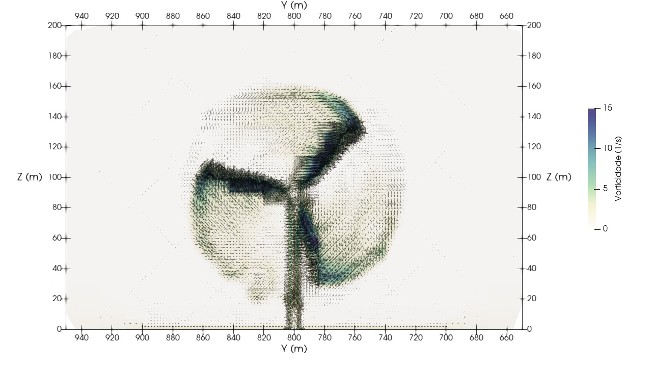
As the most elevated vorticity and gradient intensities arose near the turbine, screenshots of instantaneous vorticity contours are shown to analyze this region of the turbine. Figure 13 shows the vorticity magnitude for the ​xz​​ plane, at ​x/ D = 0​ around the turbine, where the highest vorticity values are densely scaled over the flow field. Therefore, it is possible to see that the highest vorticity densities occur mainly over the blade’s area. More specifically, as shown in Figure 14, the vorticity values tend to increase from the blade’s root to the blade’s tip direction.

Figure 13
Vectors of vorticity magnitude in the downstream position of the wind turbine.

Figure 14
Contours vorticity magnitude in the downstream position of the wind turbine.

With that said, it was aimed to comprehend which gradient had the most contribution over this area. And following the mathematical definition of vorticity, as a curl of the velocity vector, $$\mathrm{\nabla }\times \overrightarrow{u}=(\frac{\mathrm{\partial }w}{\mathrm{\partial }x}-\frac{\mathrm{\partial }v}{\mathrm{\partial }z})\mathbf{i}+(\frac{\mathrm{\partial }u}{\mathrm{\partial }z}-\frac{\mathrm{\partial }w}{\mathrm{\partial }x})\mathbf{j}+(\frac{\mathrm{\partial }v}{\mathrm{\partial }x}-\frac{\mathrm{\partial }u}{\mathrm{\partial }y})\mathbf{k}$$ ​​. As the vector field is a velocity field in a flow, this measure indicates the rotation existing in the flow.

Figure 15 depicts the instantaneous gradient components contours around the swept area, where the most significant contributions come from the velocity gradients ​∂ v / ∂ x​​ and ​∂ w / ∂ x​​ concerning the spatial variation in the flow direction (​x​​), primarily responsible for the downstream tip vortices structures Akay et al. (2014). Meanwhile, the sum of the contributions of ​∂ w / ∂ y​​ and ​∂ v / ∂ z​​, are accountable for the streamwise component of the vorticity, presenting the highest contribution on the leading edge of the blade’s tip.

Figure 15
Contours of the gradient components around the swept area.

Evaluation of power generation for single turbine

this section presents the results obtained from the temporal evolution of the torque and power of the stand-alone wind turbine. Since the geometry is incorporated into the fluid domain, by a force term in the Navier-Stokes equations, the use of the immersed boundary method the use of the immersed boundary method is taken as an advantage to obtain, with post-processing, the torque and power generated by the turbine. The steps for this evaluation consisted of:

• 1. To calculate the distance from the wind turbine rotation reference position to the center position of each Lagrangian cell:

$$r_x=x_c-{\tilde{x}}_k$$ (15)

​​$$r_y=y_c-{\tilde{y}}_k$$​​​ (16)

$$r_z=z_c-{\tilde{z}}_k$$ (17)

where ​​xc​​​​, ​yc​​​​, ​zc​​​​​​ are the rotation reference positions of the immersed boundary defined in the file input/ib.amr ​3d​​ and ​​​ ˜ x ​​ k​​​​, ​​ ˜ y ​​ k​​​​, ​​ ˜ z ​​ k​​​​​​ are the center positions of each Lagrangian cell in each direction.

• 2. To calculate the Torque through the summation in the Lagrangian space of the cross product of force and distance in ​x, y​​, and ​z​​.

$$T=\sum _{\mathrm{\Gamma }}\overrightarrow{r}\times \overrightarrow{F}$$(18)​​​

where ​F​​ represents the force magnitude of the Lagrangian field that promotes the immersed boundary rotation.

$$\overrightarrow{r}\times \overrightarrow{F}=\left|\begin{array}{ccc}\mathbf{i}& \mathbf{j}& \mathbf{k}\\ r_x& r_y& r_z\\ F_x& F_y& F_z\end{array}\right|$$(19)​​​

• 3. Calculating mechanical Torque, the mechanical Power generation is obtained using the following equation:

$$\text{Power}=\frac{T{\omega }_x\pi }{30000}$$(20)​​​

where ​​ωx​​​​​​ stands for angular velocity rotation (​rad / s​).

Figure 16 illustrates the original signals from the temporal evolution of torque, while Figure 17 depicts the original signals from the temporal evolution of power. On the abscissa axis, the scaled Torque and Power are plotted against the normalized number of iterations for a sample of about 10000 iterations after the flow is fully developed, exhibiting that the signal is periodic, thus, statistically reliable for acquiring the average of the torque and power. Hence, in terms of torque represented by Figure 16, MFSim results presented a mean and standard deviation of ​​1873.89 ± 73.90​(​​ kNm ​)​​​​while the experimental study of the NREL 5MW, Jonkman et al. (2009) showed a mean torque value of ​​1914.00​(​​ kNm ​)​​​​for the same conditions, thus the mean difference corresponds to 40.11 (​kNm​​), representing about a ​2%​ difference between both results. In the case of power generation shown by Figure 17, mean values and standard deviation for the MFSim simulation corresponds to ​1741.75 ± 69.96​ (​kW​​).

Figure 16
Torque of the NREL 5 MW.

Figure 17
Power of the NREL 5 MW.

In contrast, NREL 5MW of Jonkman et al. (2009) presented the value of ​​1805.00​(​​kW​​)​​​​, which results in a difference in generating power of ​​63.25​(​​kW​​)​​​​. Therefore, the difference in power generation between both results is about ​3.5%​, which is a pretty low difference when taking into consideration the size of the wind turbine that was applied in this work.

CONCLUSIONS

This work simulated a real-scale offshore wind turbine NREL 5 MW using large eddy simulation coupled with immersed boundary method alongside a dynamic adaptive mesh refinement. Firstly, it was decided to simulate the flow around the wind turbine with a control volume of ​1600m​​ longitudinal, ​800m​​ width, and ​600m​​ height, reaching a blockage ratio of around ​3.42%​. Then, simulations with five refinement levels over the wake were chosen in order to compare with the provided results. In terms of the comparison with the data provided from UBC, SOWFA and both TOSCA overestimate the results from MFSim in the near wake centerline for cross-sectional analysis, which could be attributed to the tower and nacelle shading effecting occurring in the near wake.

In the transition wake region, the profiles are similar to each other where most of the results have lower than ​10%​ for the whole wake width. Further downstream in the far wake region, the centerline area produced similar results among the profiles with differences lower than ​7%​ in this region. In the transition wake region, the profiles are similar to each other where most of the results have lower than ​10%​ for the whole wake width. Further downstream in the far wake region, the centerline area produced similar results among the profiles with differences lower than ​7%​ in this region. Concerning the vertical evaluation, it presented lower recovery velocities of MFSim around the hub height in the near wake compared to other profiles, which restates the simplification blade resolving geometry applied in TOSCA and SOWFA. Further downstream, in the transition wake region, the best correlation occurred between SOWFA and MFSim, from the blade’s bottom tip up to hub height, with extremely low variations that did not exceed ​3%​ between the profiles. Meanwhile, in heights above hub height, both TOSCA showed a better representation of the profile in comparison with MFSim results, where the differences were lower than ​9%​ among them. In the vertical far wake analysis, the best performance occurred around the hub area with differences, among both TOSCA and MFSim, that can reach values lower than ​1%​ variation among them.

Finally, the power production analysis demonstrated that low difference between the experimental results from NREL and MFSim, leading to a lower than ​3.5%​ difference for both torque and power generation, considering the turbine’s size applied in the simulation. Which leads to big expectations and developing of offshore turbines in countries such as Brazil.

Acknowledgements

The authors gratefully acknowledge technical and financial support from Coordenação de Aperfeiçoamento de Pessoal de Nível Superior (CAPES), Fundação de Amparo à Pesquisa do Estado de Minas Gerais (FAPEMIG), Conselho Nacional de Desenvolvimento Científico e Tecnológico (CNPq), and Petróleo Brasileiro S.A. (Petrobras). The authors are also grateful to the Graduate Program in Water Resources and Environmental Engineering at the Universidade Federal do Paraná, the Graduate Program in Mechanical Engineering at the Universidade Federal de Uberlândia, and the UBCO CFDLab of the University of British Columbia for their contribution.

References

• AKAY B, RAGNI D, SIMÃO FERREIRA C & VAN BUSSEL G. 2014. Experimental investigation of the root flow in a horizontal axis wind turbine. Wind Energy 17: 1093-1109.
• ALVES M, OLIVEIRA P & PINHO F. 2003. A convergent and universally bounded interpolation scheme for the treatment of advection. Int J Numer Methods Fluid 41: 47-75. DOI: 10.1002/fld. 428.
  » https://doi.org/10.1002/fld
• BARBI F, PIVELLO MR, VILLAR MM, SERFATY R, ROMA AM & SILVEIRA NETO A., 2018. Numerical experiments of ascending bubbles for fluid dynamic force calculations. J Braz Soc Mech Sci Eng 40: 519. https://doi.org/10.1007/s40430-018-1435-7.
  » https://doi.org/10.1007/s40430-018-1435-7
• CASTRO LP, PINHEIRO AP, VILELA V, MAGALHÃES GM, SERFATY R & VEDOVOTTO JM. 2021. Implementation of a hybrid lagrangian filtered density function-large eddy simulation methodology in a dynamic adaptive mesh refinement environment. Phys Fluids 33: 045126. DOI: 10.1063/5.0045873.
  » https://doi.org/10.1063/5.0045873
• DAMASCENO M, VEDOVOTTO JM & SILVEIRA NETO A. 2015. Turbulent inlet conditions modeling using large-eddy simulations. CMES 104: 105-132.
• DAMASCENO M, DE FREITAS SANTOS JG & VEDOVOTTO JM. 2018. Simulation of turbulent reactive flows using a fdf methodology - advances in particle density control for normalized variables. Comput Fluids 170: 128-140.
• EDELENBOSCH O, KERMELI K, CRIJNS-GRAUS W, WORRELL E, BIBAS R, FAIS B, FUJIMORI S, KYLE P, SANO F & VAN VUUREN D. 2017. Comparing projections of industrial energy demand and greenhouse gas emissions in long-term energy models. Energy 122: 701-710.
• FRANDSEN S, BARTHELMIE R, PRYOR S, RATHMANN O, LARSEN S, HØJSTRUP J & THØGERSEN M. 2006. Analytical modelling of wind speed deficit in large offshore wind farms. Wind Energy 9(1): 39-53.
• GERMANO M, PIOMELLI U, MOIN P & CABOT WH. 1991. A dynamic subgrid-scale eddy viscosity model. Phys Fluids A: Fluid Dynamics 3(7): 1760-1765. DOI: 10.1063/1.857955.
  » https://doi.org/10.1063/1.857955
• HOU G, WANG J & LAYTON A. 2012. Numerical methods for fluid-structure interaction - a review. Comm Comput Phys 12(2): 337-377. 10.4208/cicp.291210.290411s.
• IACCARINO G & VERZICCO R. 2003. Immersed boundary technique for turbulent flow simulations. Appl Mech Rev 56(4): 331. DOI: 10.1115/1.1563627.
  » https://doi.org/10.1115/1.1563627
• JENSEN N. 1983. A note on wind generator interaction. Risø-M, n. 2411. Risø National Laboratory.
• JEONG J & HUSSAIN F. 1995. On the identification of a vortex. J Fluid Mech 285: 69-94.
• JONKMAN J, BUTTERFIELD S, MUSIAL W & SCOTT G. 2009. Definition of a 5 -mw reference wind turbine for offshore system development. Golden Colorado National Renewable Energy Laboratory. DOI: 10.2172/947422.
• KILKIŞ Ş, KRAJAČIĆ G, DUIĆ N, ROSEN MA & AL-NIMR MA. 2018. Advancements in sustainable development of energy water and environment systems. Energ Convers Manag 176: 164-183.
• LARSEN G. 1988. A Simple Wake Calculation Procedure. Risø-M, n. 2760. Risø National Laboratory.
• LEUNG D & YANG Y. 2012. Wind energy development and its environmental impact: A review. Renew Sustain Energy Rev 16(1): 1031-1039.
• LILLY DK. 1992. A proposed modification of the germano subgrid-scale closure method. Physics of Fluids A: Fluid Dynamics 4(3): 633-635.
• MELO R, KINOSHITA D, VILLAR M, SERFATY R & SILVEIRA-NETO A. 2018. Simulation of thermal transfer using the immersed boundary method and adaptive mesh. DOI: 10.1615/THMT-18.1040
• MELO RRDS. 2017. Modelagem e simulação de escoamentos turbulentos com efeitos térmicos utilizando a metodologia da fronteira imersa e malha adaptativa. Tese de Doutorado em Engenharia Mecânica, Universidade Federal de Uberlândia.
• MITTAL R & IACCARINO G. 2005. Immersed Boundary Methods. Ann Rev Fluid Mech 37: 239-261. DOI: 10.1146/annurev.fluid.37.061903.175743.
  » https://doi.org/10.1146/annurev.fluid.37.061903.175743
• MO JO, CHOUDHRY A, ARJOMANDI M, KELSO R & LEE YH. 2013. Effects of wind speed changes on wake instability of a wind turbine in a virtual wind tunnel using large eddy simulation. J Wind Eng Industr Aerodynamic 117: 38-56. http://www.sciencedirect.com/science/article/pii/S0167610513000718.
• MOHAMMADI M, SOTIROPOULOS F & BRINKERHOFF J. 2018. Moving least squares reconstruction for sharp interface immersed boundary methods: Mls reconstruction in the immersed boundary method. Int J Numer Methods Fluids 90(11): 6117-6138 DOI: 10.1002/fld.4711.
  » https://doi.org/10.1002/fld.4711
• MORALES FAP, SERFATY R, VEDOVOTTO JM, CAVALLINI A, VILLAR MM & DA SILVEIRA NETO A. 2023. Fluid-structure interaction with a finite element-immersed boundary approach for compressible flows. Ocean Eng 290: 115755.
• MOTA PHA, VEDOVOTTO JM & SILVEIRA NETO A. 2023. Assessment of critical brine disposal operations conditions by cfd modeling and a kriging metamodel. Environ Fluid Mech 23(6): 1573-1600. DOI: 10.1007/s10652-023-09911-7.
  » https://doi.org/10.1007/s10652-023-09911-7
• NADERI S, PARVANEHMASIHA S & TORABI F. 2018. Modeling of horizontal axis wind turbine wakes in horns rev offshore wind farm using an improved actuator disc model coupled with computational fluid dynamic. Energy Conv Manag 171: 953-968. https://www.sciencedirect.com/science/article/pii/S0196890418306538.
• NETO HR, CAVALINI A, VEDOVOTO J, NETO AS & RADE D. 2019. Influence of seabed proximity on the vibration responses of a pipeline accounting for fluid-structure interaction. Mech Syst Signal Proc 114: 224-238.
• PESKIN CS. 2002. The immersed boundary method. Acta Numerica 11: 479-517. 10.1017/S0962492902000077.
• PINHEIRO AP, RYBDYLOVA O, ZUBRILIN IA, SAZHIN SS, SACOMANO FILHO FL & VEDOVOTTO JM. 2021. Modelling of aviation kerosene droplet heating and evaporation using complete fuel composition and surrogates. Fuel 305: 121564. https://doi.org/10.1016/j.fuel.2021.121564.
  » https://doi.org/10.1016/j.fuel.2021.121564
• PINHEIRO AP, VEDOVOTO JM, DA SILVEIRA NETO A & VAN WACHEM BG. 2019. Ethanol droplet evaporation: Effects of ambient temperature pressure and fuel vapor concentration. Int J Heat Mass Transf 143: 118472. https://doi.org/10.1016/j.ijheatmasstransfer.2019.118472
  » https://doi.org/10.1016/j.ijheatmasstransfer.2019.118472
• REGODESEVES PG & MORROS CS. 2021. Numerical study on the aerodynamics of an experimental wind turbine: Influence of nacelle and tower on the blades and near-wake. Energ Conv Manag 237: 114110. https://doi.org/10.1016/j.enconman.2021.114110.
  » https://doi.org/10.1016/j.enconman.2021.114110
• SANTOS JGDF. 2019. Mathematical and computational modeling of gas-solid flows in dynamic adaptive mesh. Dissertação de Mestrado em Engenharia Mecânica, Universidade Federal de Uberlândia. (Unpublished).
• SEDAGHATIZADEH N, ARJOMANDI M, KELSO R, CAZZOLATO B & GHAYESH MH. 2018. Modelling of wind turbine wake using large eddy simulation. Renew Energy 115: 1166-1176. https://doi.org/10.1016/j.renene.2017.09.017
  » https://doi.org/10.1016/j.renene.2017.09.017
• SOTIROPOULOS F & YANG X. 2014. Immersed boundary methods for simulating fluid-structure interaction. Progr Aerosp Sci 65: 1-21. DOI: 10.1016/j.paerosci.2013.09.003.
  » https://doi.org/10.1016/j.paerosci.2013.09.003
• SOUZA PRC, NETO HR, VILLAR MM, VEDOVOTTO JM, CAVALINI AA & NETO AS. 2022. Multi-phase fluid-structure interaction using adaptive mesh refinement and immersed boundary method. J Braz Soc Mech Sci Eng 44(5): 250. DOI: 10.1007/s40430-022-03417-x.
  » https://doi.org/10.1007/s40430-022-03417-x
• STIPA S, AJAY A, ALLAERTS D & BRINKERHOFF J. 2023. Tosca - an open-source finite-volume les environment for wind farm flows. Wind Energy Sci Discussions 9(2): 297-320. https://doi.org/10.5194/wes-9-297-2024.
  » https://doi.org/10.5194/wes-9-297-2024
• SYED AHMED KABIR IF & NG E. 2019. Effect of different atmospheric boundary layers on the wake characteristics of nrel phase vi wind turbine. Renew Energ 130: 1185-1197. https://doi.org/10.1016/j.renene.2018.08.083.
  » https://doi.org/10.1016/j.renene.2018.08.083
• UZGOREN E, SINGH R, SIM J & SHYY W. 2007. Computational modeling for multiphase flows with spacecraft application. Progr Aerosp Sci 43(5-6): 138-192. DOI: 10.1016/j.paerosci.2007.06.003.
  » https://doi.org/10.1016/j.paerosci.2007.06.003
• VEDOVOTO JM, SERFATY R & SILVEIRA NETO A. 2015. Mathematical and Numerical Modeling of Turbulent Flows. An Acad Bras Cienc 87: 1195-1232. https://doi.org/10.1590/0001-3765201520140510.
  » https://doi.org/10.1590/0001-3765201520140510
• VERMEER L, SØRENSEN J & CRESPO A. 2003. Wind turbine wake aerodynamics. Progr Aerosp Sci 39(6-7): 467-510.
• VILLAR M. 2007. Análise numérica detalhada de escoamentos multifásicos bidimensionais. Tese de Doutorado em Engenharia Mecânica, Universidade Federal de Uberlândia.
• WANG L, TAN A, CHOLETTE M & GU Y. 2016. Comparison of the effectiveness of analytical wake models for wind farm with constant and variable hub heights. Energy Conv Manag 124: 189-202. DOI: 10.1016/j.enconman.2016.07.017.
  » https://doi.org/10.1016/j.enconman.2016.07.017
• WANG Y, WANG L, JIANG Y & SUN X. 2022. A new method for prediction of power coefficient and wake length of a horizontal axis wind turbine based on energy analysis. Energ Conv Manag 252: 115121. https://doi.org/10.1016/j.enconman.2021.115121.
  » https://doi.org/10.1016/j.enconman.2021.115121
• WANG Z, FAN J & LUO K. 2008. Combined multi-direct forcing and immersed boundary method for simulating flows with moving particles. Int J Multiphase Flow 34(3): 283-302.

Publication Dates

• Publication in this collection
  20 Oct 2025
• Date of issue
  2025

History

• Received
  16 Aug 2024
• Accepted
  29 Mar 2025